Examples
This page highlights several examples on how dynesty
can be used in practice, illustrating both simple and more advanced
aspects of the code. Jupyter notebooks containing more details are available
on Github.
Gaussian Shells
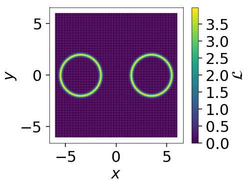
The “Gaussian shells” likelihood is a useful test case for illustrating the ability of nested sampling to deal with oddly-shaped distributions that can be difficult to probe with simple random-walk MCMC methods.
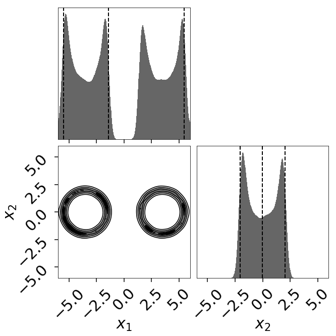
dynesty returns the following posterior estimate:
Eggbox
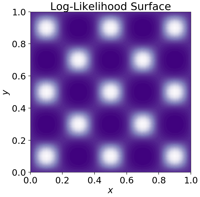
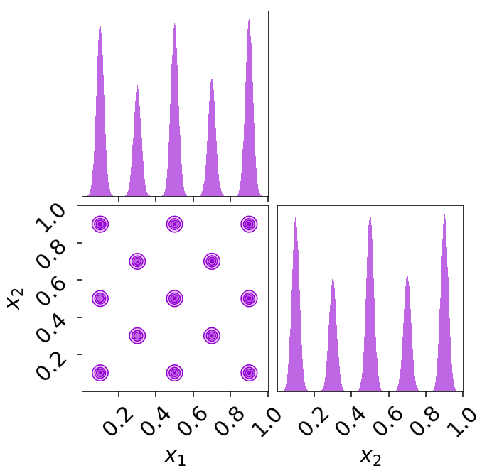
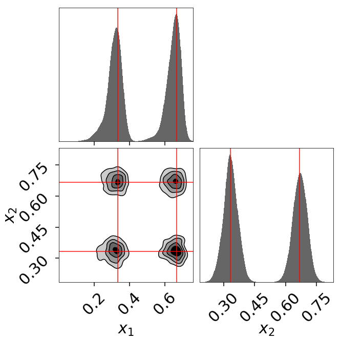
The “Eggbox” likelihood is a useful test case that demonstrates Nested Sampling’s ability to properly sample/integrate over multi-modal distributions.
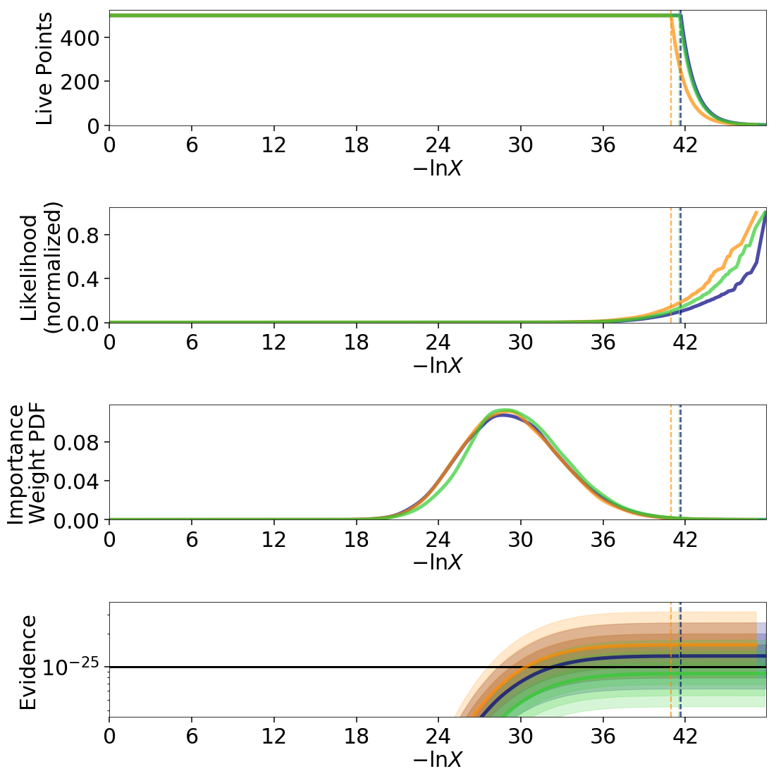
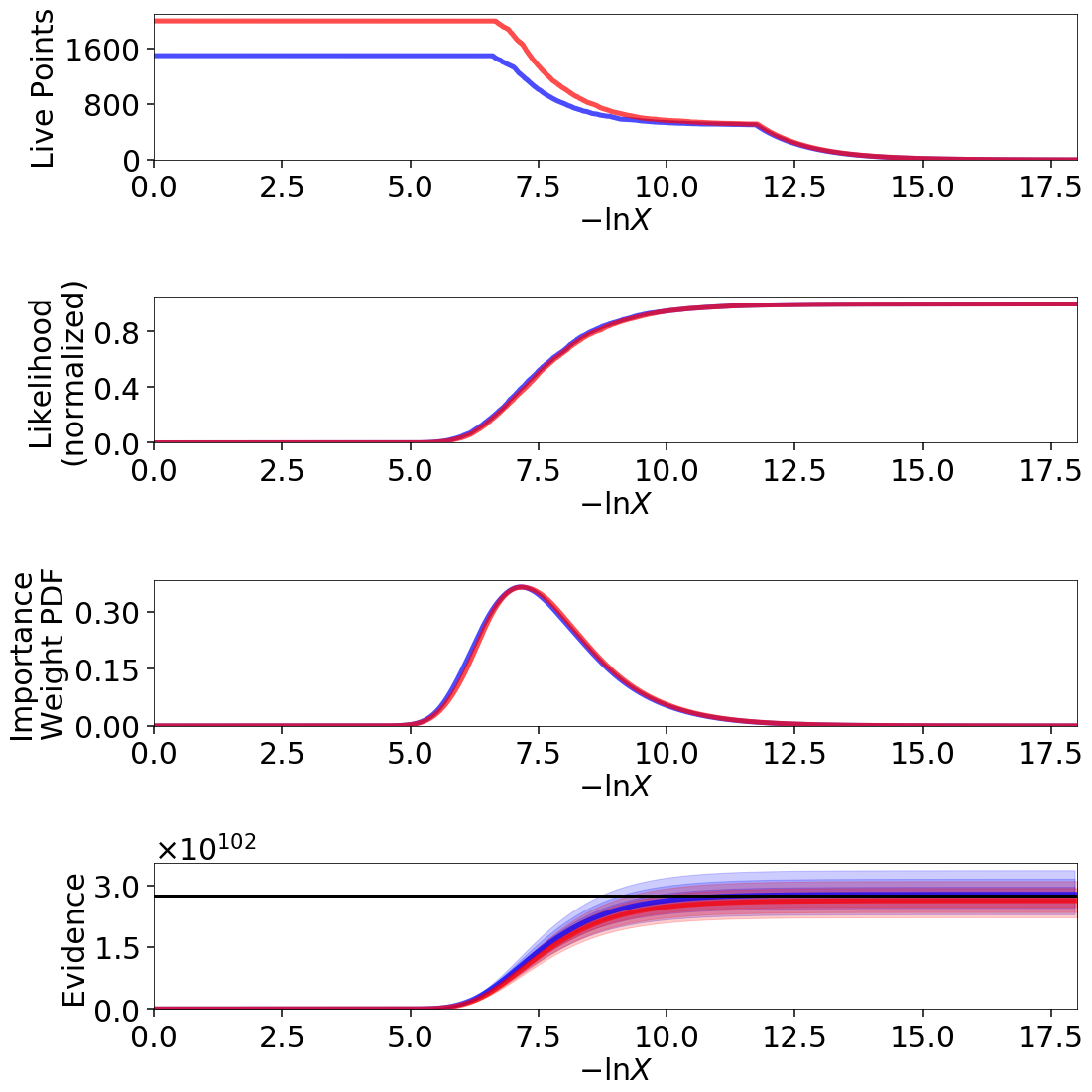
The evidence estimates from two independent runs look reasonable:
The posterior estimate also looks quite good:
Exponential Wave
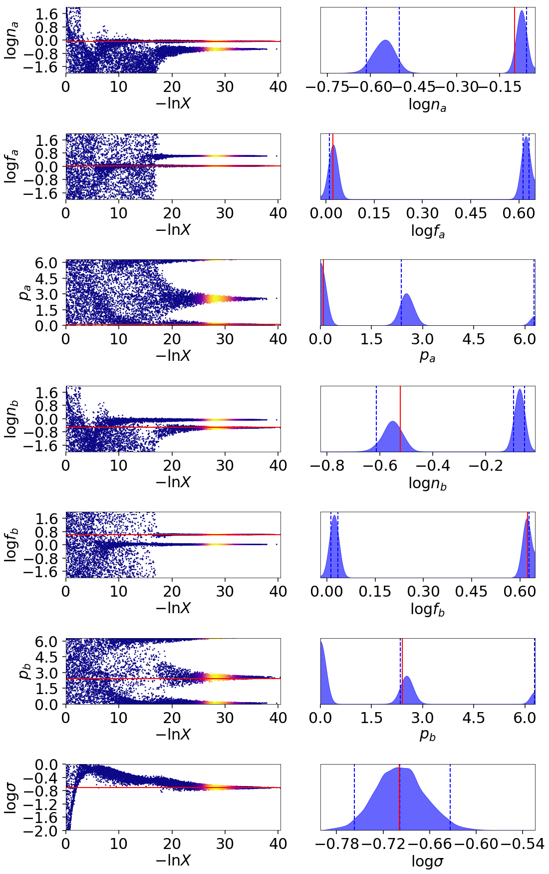
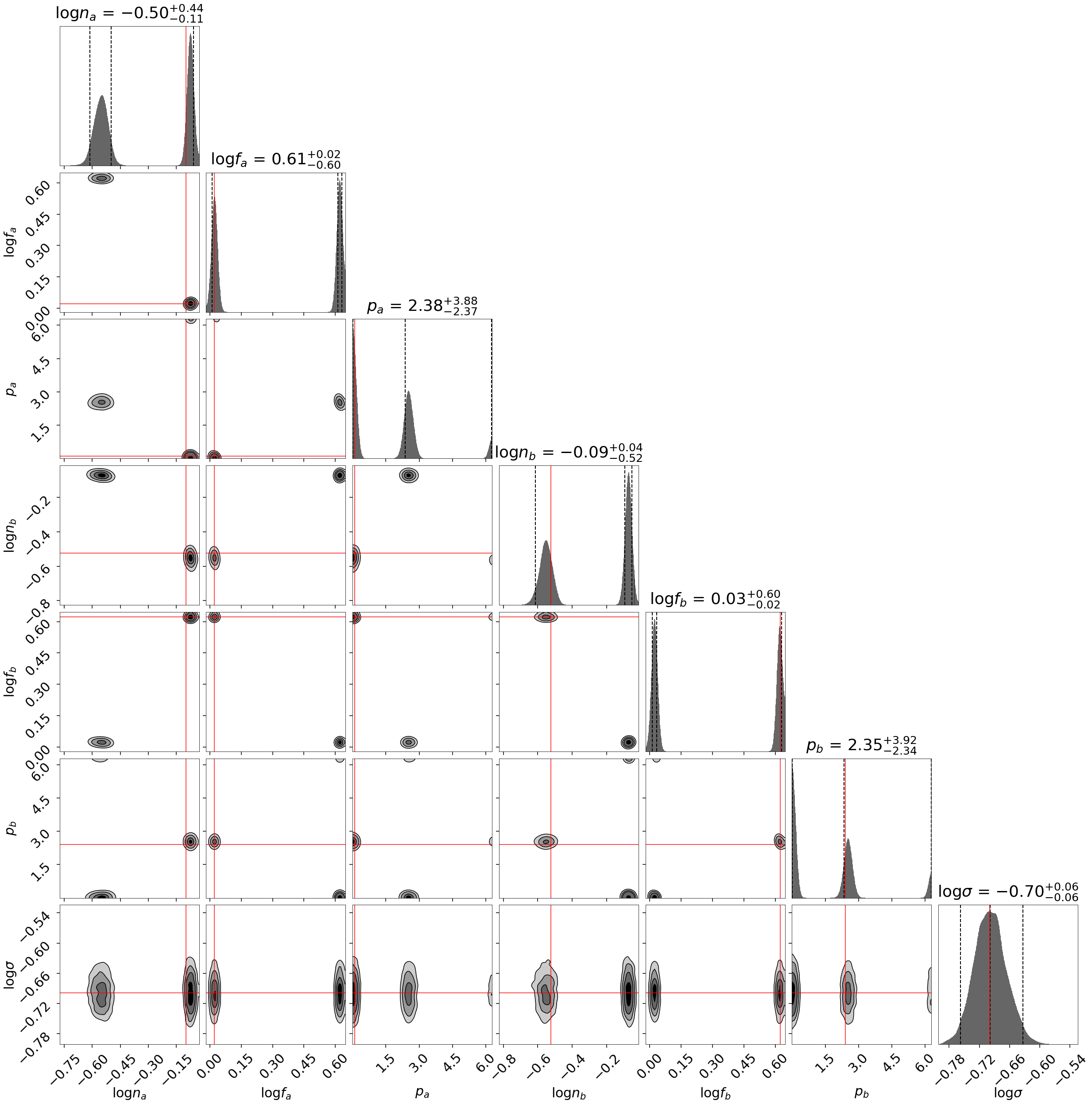
This toy problem was originally suggested by suggested by Johannes Buchner for being multimodal with two roughly equal-amplitude solutions. We are interested in modeling periodic data of the form:
where \(x\) goes from \(0\) to \(2\pi\).
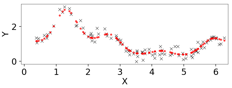
This model has six free parameters controling the relevant amplitude, period, and phase of each component (which have periodic boundary conditions). We also have a seventh, \(\sigma\), corresponding to the amount of scatter.
The results are shown below.
Linear Regression
Linear regression is ubiquitous in research. In this example we’ll fit a line
to data where the error bars have been over/underestimated by some fraction
of the observed value \(f\) and need to be decreased/increased.
Note that this example is taken directly from the emcee documentation.
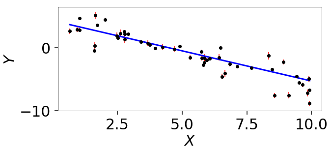
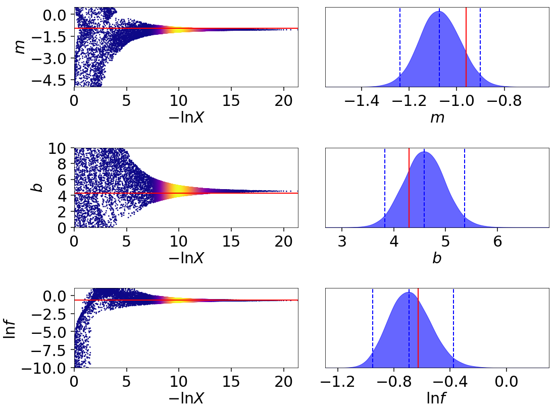
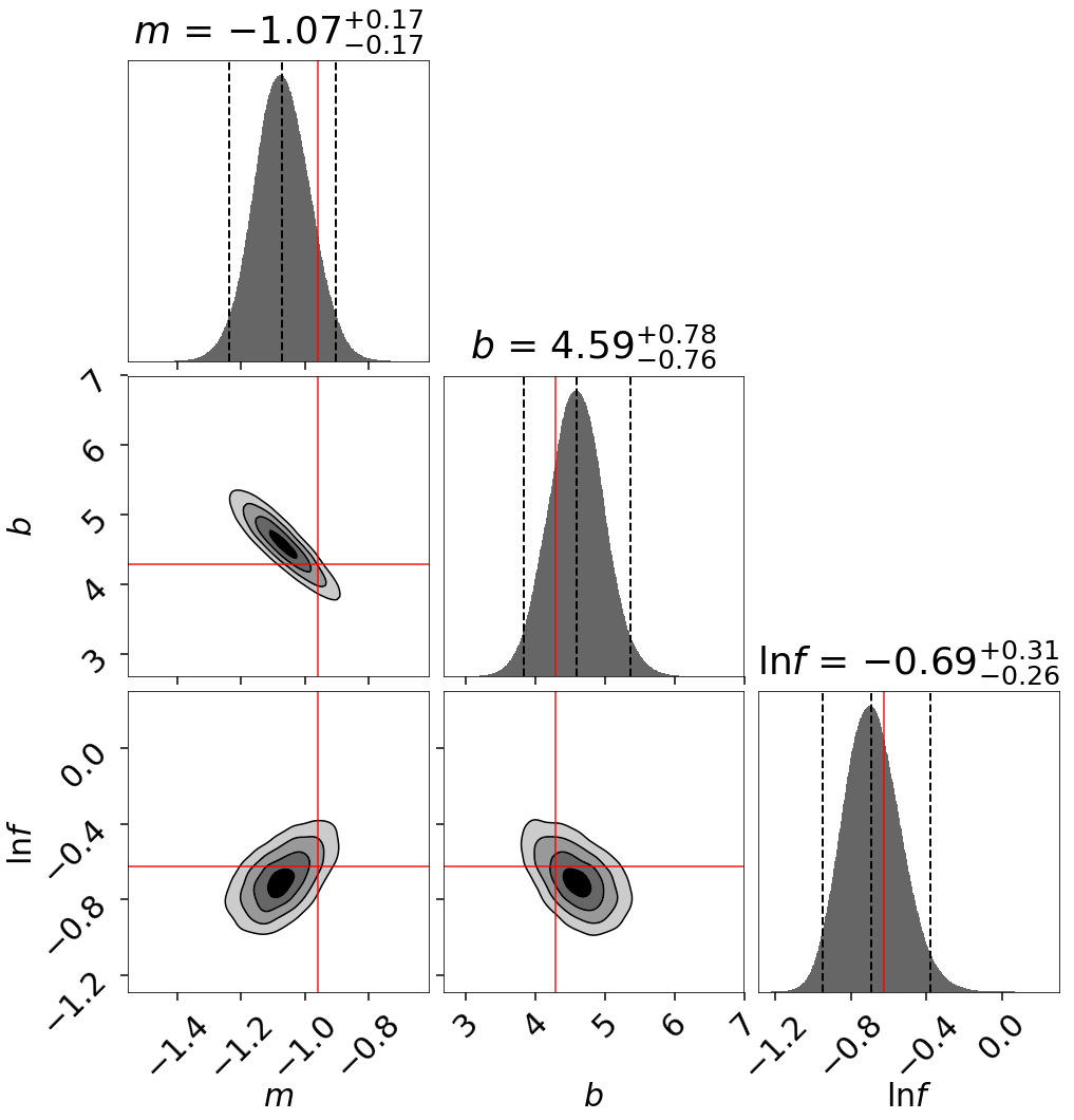
The trace plot and corner plot show reasonable parameter recovery.
Hyper-Pyramid
One of the key assumptions of Static Nested Sampling (extended by Dynamic Nested Sampling) is that we “shrink” the prior volume \(X_i\) at each iteration \(i\) as
at each iteration with \(t_i\) a random variable with distribution \(\textrm{Beta}(K, 1)\) where \(K\) is the total number of live points. We can empirically test this assumption by using functions whose volumes can be analytically computed directly from the position/likelihood of a sample.
One example of this is the “hyper-pyramid” function from Buchner (2014).

We can compare the set of samples generated from dynesty
with the expected theoretical shrinkage
using a Kolmogorov-Smirnov (KS) Test.
When sampling uniformly from a set of bounding ellipsoids, we expect to be
more sensitive to whether they fully encompass the bounding volume. Indeed,
running on default settings in higher dimensions yields shrinkages that
are inconsistent with our theoretical expectation (i.e. we shrink too fast):

If bootstrapping is enabled so that ellipsoid expansion factors are determined “on the fly”, we can mitigate this problem:

Alternately, using a sampling method other than 'unif' can also avoid this
issue by making our proposals less sensitive to the exact size/coverage
of the bounding ellipsoids:

LogGamma
The multi-modal Log-Gamma distribution is useful for stress testing the effectiveness of bounding distributions since it contains multiple modes coupled with long tails.
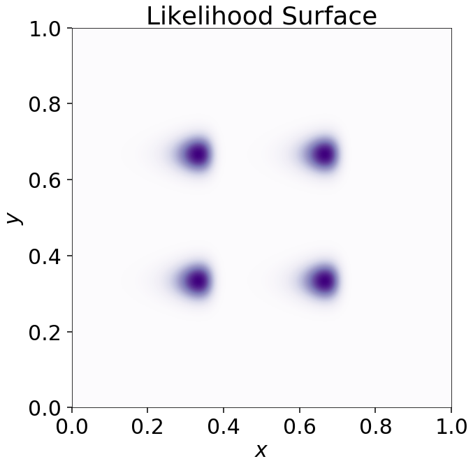
dynesty is able to sample from this distribution in \(d=2\) dimensions
without too much difficulty:
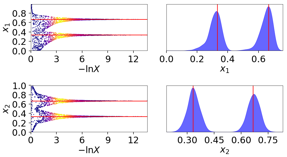
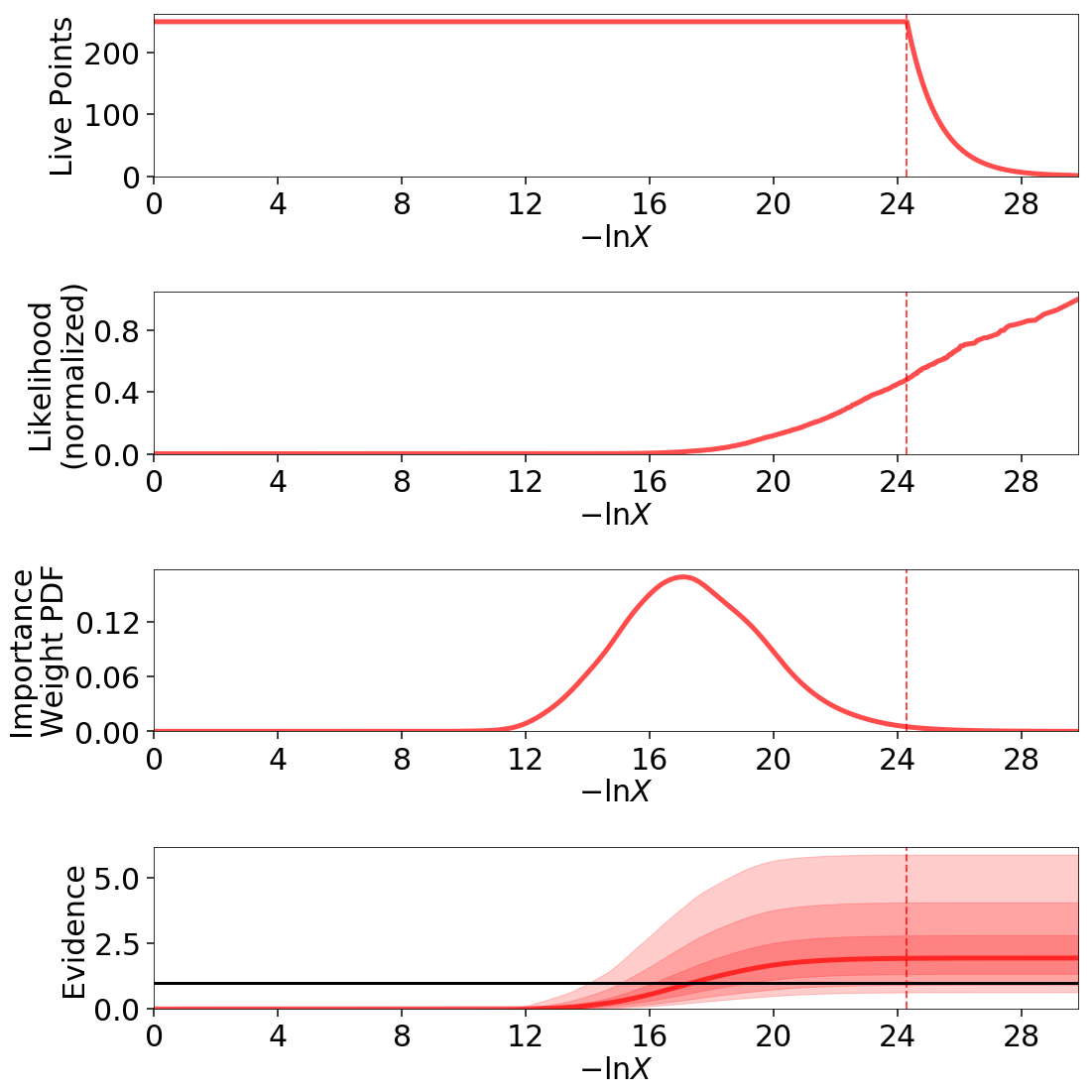
Although the analytic estimate of the evidence error diverges (requiring us to compute it numerically following Nested Sampling Errors), we are able to recover the evidence and the shape of the posterior quite well:
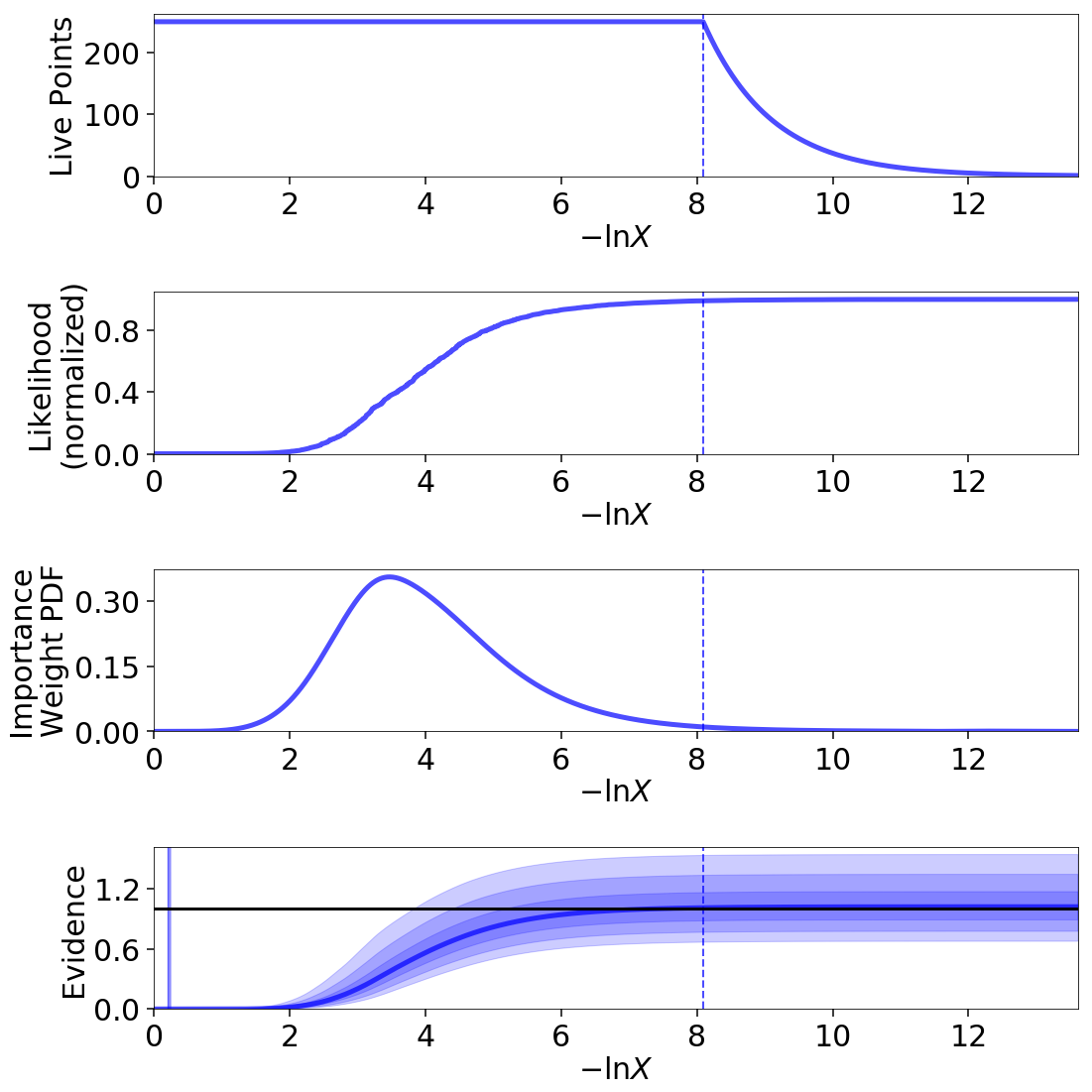
Our results in \(d=10\) dimensions are also consistent with the expected theoretical value:
200-D Normal
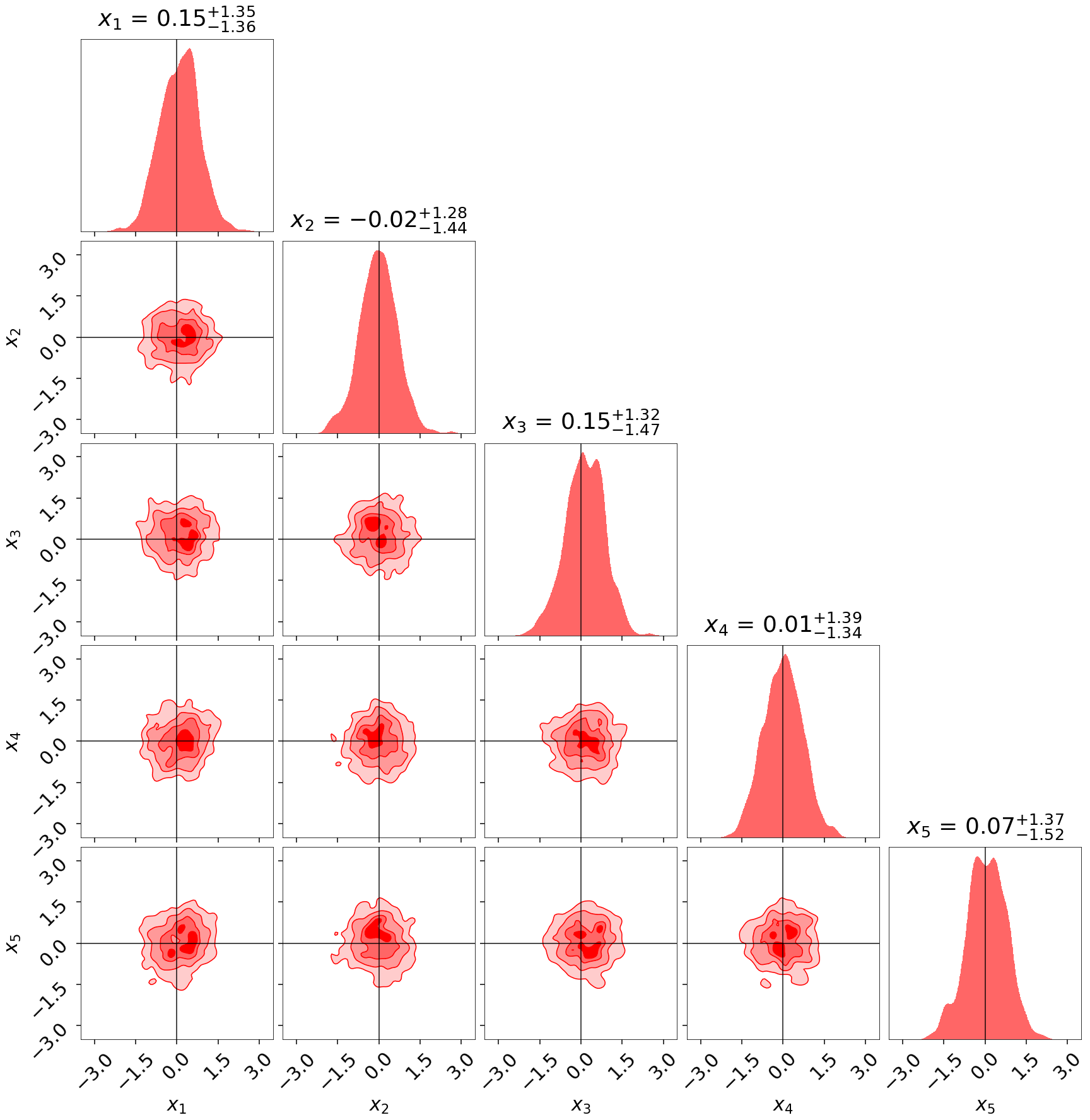
We examine the impact of gradients for sampling from high-dimensional
problems using a 200-D iid normal distribution with an associated
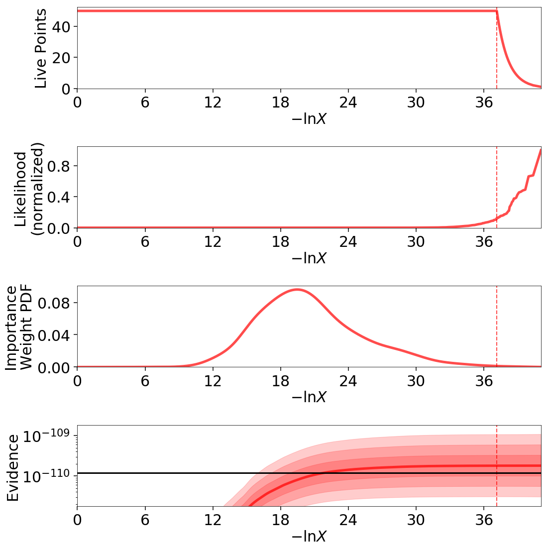
200-D iid normal prior. With Hamiltonian slice sampling ('hslice'), we find
we are able to recover the appropriate evidence:
Our posterior recovery also appears reasonable, as evidenced by the small snapshot below:
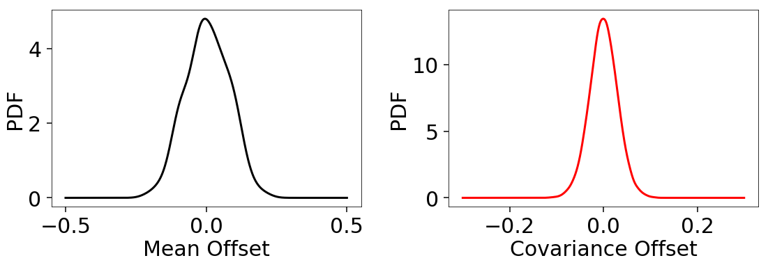
We also find unbiased recovery of the mean and covariances in line with the accuracy we’d expect given the amount of live points used:

Importance Reweighting
Nested sampling generates a set of samples and associated importance weights,
which can be used to estimate the posterior. As such, it is trivial to
re-weight our samples to target a slightly different distribution using
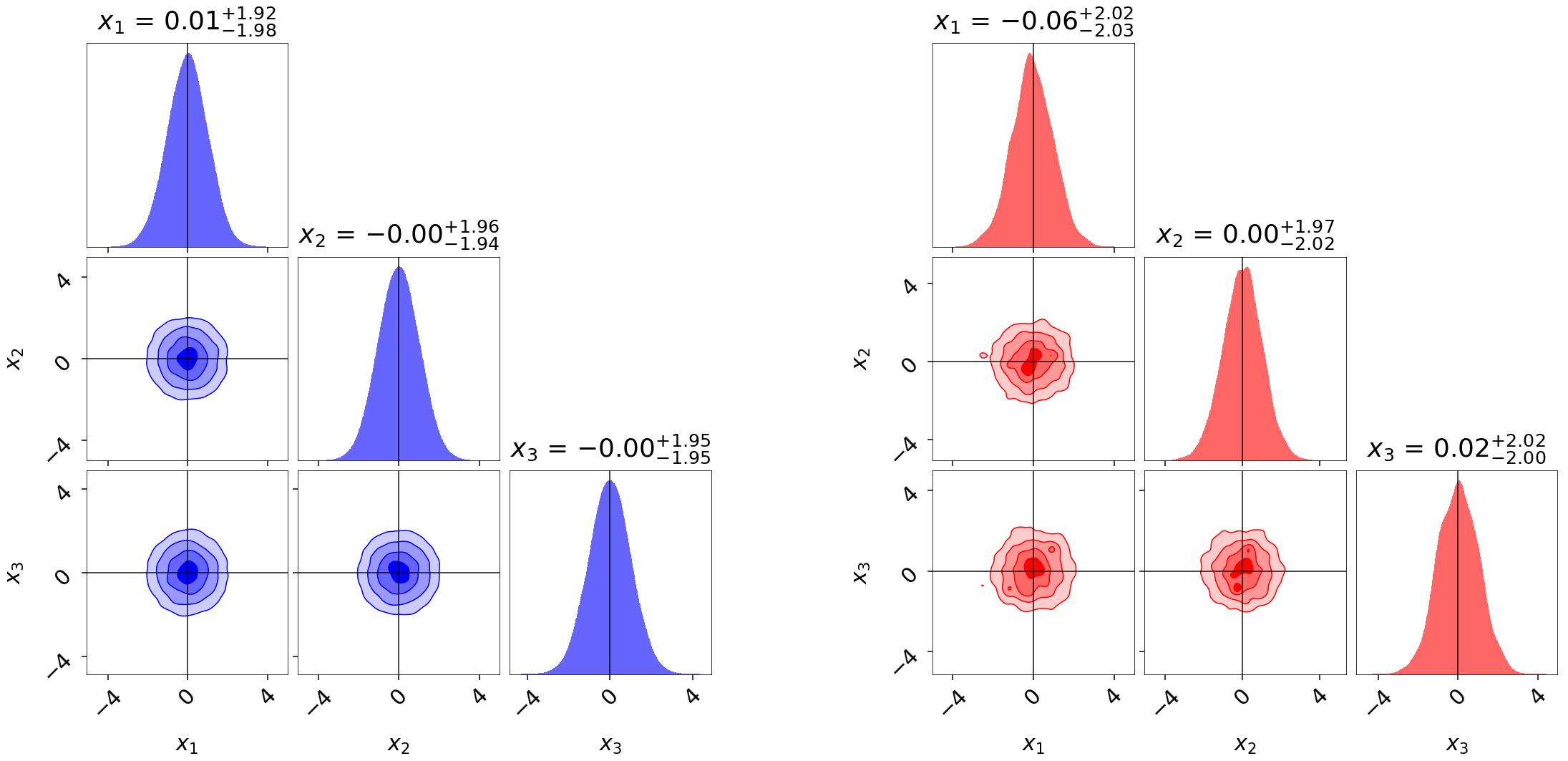
importance reweighting. To illustrate this, we run dynesty on two 3-D
multivariate Normal distributions with and without strong covariances.
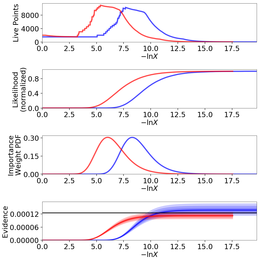
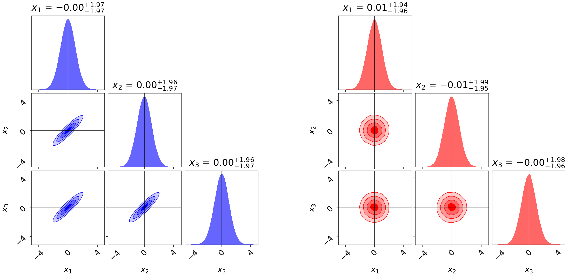
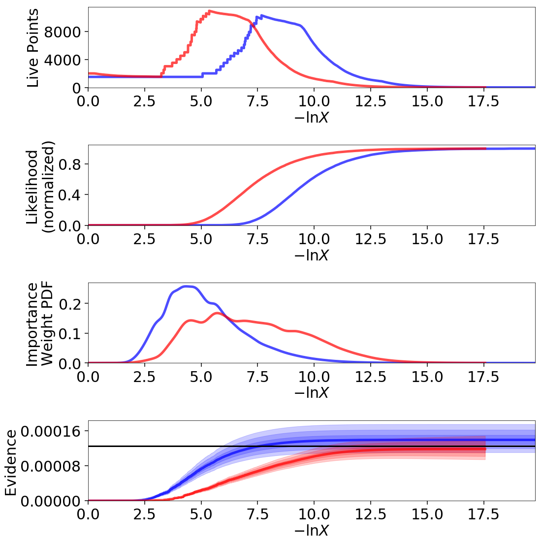
We then use the built-in utilities in dynesty to reweight each set of
samples to approximate the other distribution. Given that both samples have
non-zero coverage over each target distribution, we find that the results
are quite reasonable:

Noisy Likelihoods
It is possible to sample from noisy likelihoods in
dynesty just like with MCMC provided they are unbiased. While there
are additional challenges to sampling from noisy likelihood surfaces,
the largest is the fact that over time we expect the likelihoods to be biased
high due to the baised impact of random fluctuations on sampling: while
fluctuations to lower values get quickly replaced, fluctuations to higher
values can only be replaced by fluctuations to higher values elsewhere. This
leads to a natural bias that gets “locked in” while sampling, which can
substantially broaden the likelihood surface and thus the inferred posterior.
We illustrate this by adding in some random noise to a 3-D iid Normal distribution. While the allocation of samples is almost identical, the estimated evidence is substantially larger and the posterior substantially broader due to the impact of these positive fluctuations.
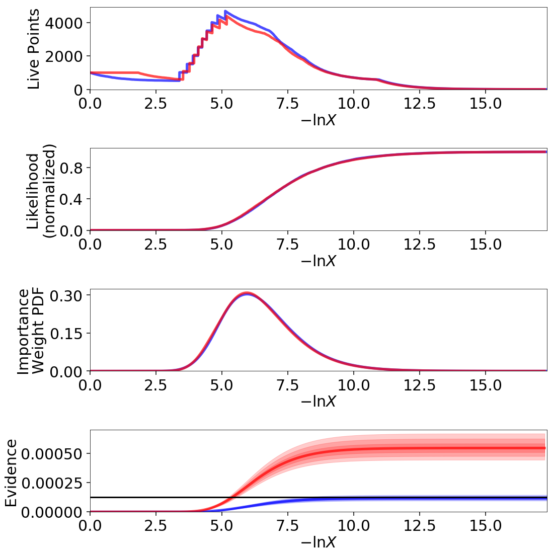
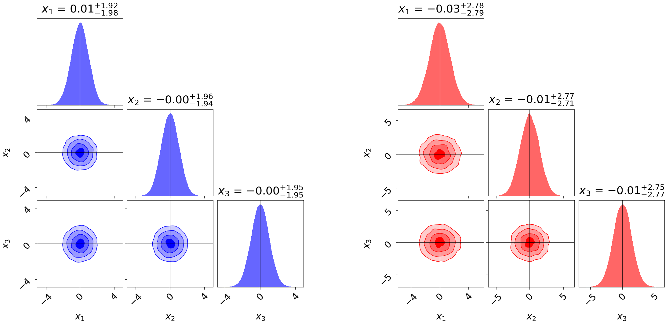
If we know the “true” underlying likelihood, it is straightforward to use Importance Reweighting to adjust the distribution to match:
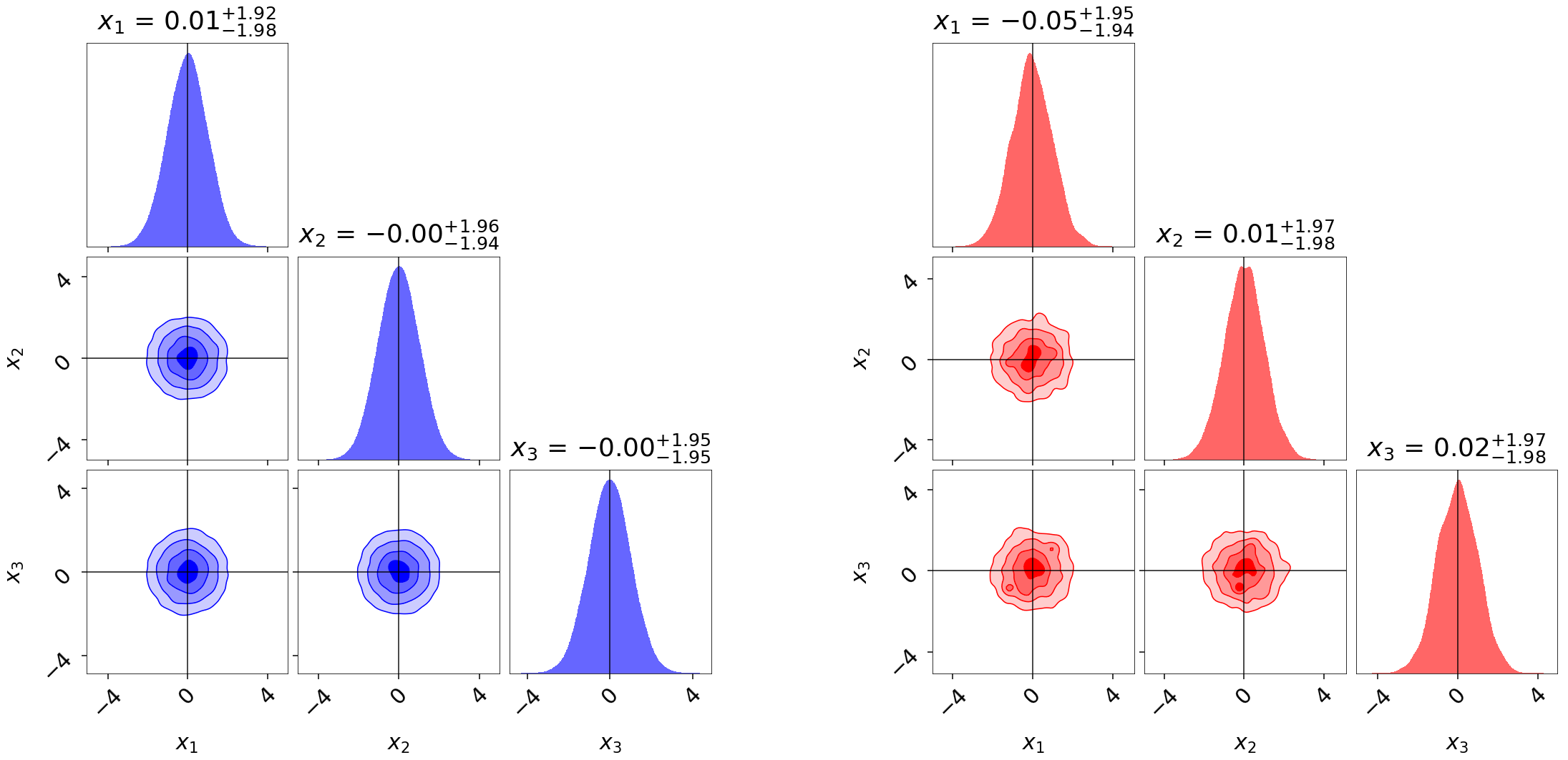
However, in most cases these are not available. In that case, we have to rely on being able to generate multiple realizations of the noisy likelihood at the set of evaluated positions in order to obtain more accurate (but still noisy) estimates of the underlying likelihood. These can then be used to get an estimate of the true distribution through the appropriate importance reweighting scheme:
