Nested Sampling Errors
Nested Sampling has two main sources of error. The first is the statistical errors associated with uncertainties on the prior volume \(X_i\) at a given iteration \(i\). This leads to uncertainties on the estimated log-evidence \(\ln \hat{\mathcal{Z}}\) and the associated posterior importance weights \(\hat{p}_i\). The second is the sampling errors associated with replacing the integral over the parameters \(\boldsymbol{\Theta}\) of interest with a single sample \(\boldsymbol{\Theta}_i\) from the corresponding iso-likelihood contour defined by \(\mathcal{L}(\boldsymbol{\Theta}) = \lambda_i\).
One of the neat features of Nested Sampling is that we are able to probe
these uncertainties within the same run used to compute the results. We
exploit this fact within dynesty in two ways. The first is a set of
functions within utils that can inject these errors into Nested
Sampling Results. This allows users to compute realistic
error budgets without going through the tedious task of computing many Nested
Sampling runs. The second way is through the default Dynamic Nested Sampling
stopping_function(), which uses this error budget
when deciding whether to stop adding samples.
This page will go through some of the main results associated with deriving
both exact and approximate error budgets for different aspects of Nested
Sampling and show how to implement them in dynesty.
Approximate Evidence Errors
In a given Static Nested Sampling run with \(K\) live points, the prior volume evolves as:
As mentioned in Priors in Nested Sampling, the “information” gained from moving from the prior \(\pi(\boldsymbol{\Theta})\) to the posterior \(P(\boldsymbol{\Theta})\) can be quantified using the KL Divergence between the two distributions:
This can be re-written in terms of an integral over the prior volume as:
where \(\mathcal{Z}\) is the again the Bayesian evidence.
As such, the number of steps \(N\) needed to integrate over the majority of the posterior starting from the prior subject to some \(\Delta \ln \hat{\mathcal{Z}}\) (see Stopping Criteria) must scale with \(H\). We also know that \(N\) should scale inversely with the typical \(\Delta \ln X\). This gives us that the expected number of steps \(\mathbb{E}[N]\) goes as
Assuming that the number of steps follows a Poisson distribution, we then expect the variance \(\mathbb{V}[N]\) should also scale as
Since the the prior volumes compress exponentially, the uncertainty on \(N\) leads to exponential uncertainty in \(X\) (and hence \(\mathcal{Z}\)) at a given iteration, so this uncertainty actually contributes in \(\ln \mathcal{Z}\) rather than \(\mathcal{Z}\). The rough uncertainty in \(\ln \mathcal{Z}\) is then:
This approximation can be extended to Dynamic Nested Sampling runs by exploiting the fact that
where we take \(\ln \hat{\mathcal{Z}}_0 = 0\). Approximating \(\mathbb{V}[\Delta \ln \hat{\mathcal{Z}_i}]\) as
shows that the contribution to the error at each iteration is based on the differential change in information \(\Delta H_i\) multiplied by the differential change in log-prior volume \(\Delta \ln X\), which we can substitute with \(\Delta \ln X_i\). This gives us:
These are the errors that are returned by default in the output stderr
statements and output Results instances and used in
plotting functions.
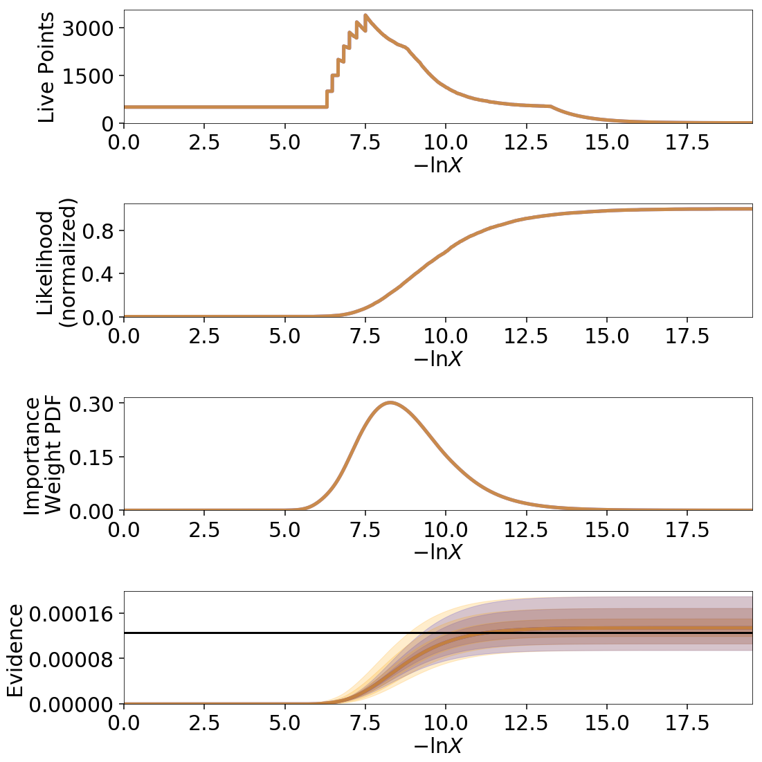
As an example, here’s a comparison among two different runs to showcase how the approximate errors take into account varying numbers of live points (and the associated changes in prior volume) throughout a given Nested Sampling run:
# static nested sampling
sampler = dynesty.NestedSampler(loglikelihood, prior_transform, ndim,
                                bound='single', nlive=1000)
sampler.run_nested()
res = sampler.results
sys.stderr.write('\n')

sampler.reset()
sampler.run_nested(dlogz=0.01)
res2 = sampler.results
sys.stderr.write('\n')

# dynamic nested sampling
dsampler = dynesty.DynamicNestedSampler(loglikelihood, prior_transform,
                                        ndim, bound='single')
dsampler.run_nested(maxiter=res2.niter+res2.nlive, use_stop=False)
dres = dsampler.results
Out:
iter: 8973 | +1000 | bound: 8 | nc: 1 | ncall: 47632 | eff(%): 20.938 |
loglstar:   -inf < -0.300 <    inf | logz: -9.169 +/-  0.097 |
dlogz:  0.001 >  1.009
iter: 13175 | +1000 | bound: 14 | nc: 1 | ncall: 54140 | eff(%): 26.182 |
loglstar:   -inf < -0.294 <    inf | logz: -8.852 +/-  0.084 |
dlogz:  0.000 >  0.010
iter: 14175 | batch: 7 | bound: 35 | nc: 1 | ncall: 39494 |
eff(%): 35.892 | loglstar: -5.792 < -0.329 < -0.645 |
logz: -8.930 +/-  0.116 | stop:    nan
The differences among the results illustrate how the location where samples are allocated can significantly affect the error budget, as discussed in Dynamic Nested Sampling.
Statistical Uncertainties
This section deals primarily with the statistical uncertainties associated with Nested Sampling. These arise from the probabilistic way a prior volume \(X_i\) is assigned to a particular sample \(\boldsymbol{\Theta}_i\) and iso-likelihood contour \(\mathcal{L}_i\).
Order Statistics
Nested Sampling works thanks to the “magic” of order statistics. At the start of a Nested Sampling run, we sample \(K\) points from the prior \(\pi(\boldsymbol{\Theta})\) with likelihoods \(\lbrace \mathcal{L}_1, \dots, \mathcal{L}_{K} \rbrace\) and associated prior volumes \(\lbrace X_1, \dots, X_K \rbrace\). We then want to pick the point with the smallest (worst) likelihood \(\mathcal{L}_{(1)}\) out of the ordered set \(\lbrace \mathcal{L}_{(1)}, \dots, \mathcal{L}_{(K)} \rbrace\) from smallest to largest. These likelihoods correspond to an ordered set of prior volumes \(\lbrace X_{(1)}, \dots, X_{(K)} \rbrace\), where the likelihoods and prior volumes are inversely ordered such that \(\mathcal{L}_{(i)} \leftrightarrow X_{(K-i+1)}\).
What is this prior volume? Since all the points were drawn from the prior, the probability integral transform (PIT) tells us that the corresponding prior volumes are uniformly distributed random variables such that
where \(\textrm{Unif}\) is the standard Uniform distribution. It can be shown through the Renyi representation (and other methods) that the set of ordered uniform random variables (the prior volumes) can be jointly represented by \(K+1\) standard Exponential random variables
where \(\textrm{Expo}\) is the standard Exponential distribution.
Prior Volumes and Order Statistics
Constant Number of Live Points
The marginal distribution of the prior volume \(X_{(K)}\) associated with the live point with the lowest likelihood \(\mathcal{L}_{(1)}\) is
where \(\textrm{Beta}(\alpha, \beta)\) is the Beta distribution with concentration parameters \((\alpha, \beta)\).
Once we replace a live point with a new live point drawn from the prior with \(\mathcal{L}_i \geq \mathcal{L}_{(1)}\), we now want to do the same procedure again. Using the same logic as above, we know that our prior volumes must be independently and identically (i.i.d.) uniformly distributed within the previous volume since we just replaced the worst point with a new independent draw. At a given iteration \(i\) the prior volume associated of the live point with the worst likelihood is then
This means that we’re compressing by a factor of
\(\mathbb{E}[t_i] = K/(K+1)\) at each iteration. This result allows us to
simulate the change in prior volume using numerical methods such as
numpy.random.beta.
Increasing Number of Live Points
In the Dynamic Nested Sampling case at a given iteration we can add in new live points so that the number of effective live points \(K_i > K_{i-1}\). Since all the samples are i.i.d. by construction, we end up with the modified result
Decreasing Number of Live Points
In the case where the number of live points are decreasing, we are now directly sampling “down” the set of order statistics \(\lbrace X_{(1)}, \dots, X_{(K_j)} \rbrace\) described above. If at iteration \(i > j\) we have \(K_i < K_{i+1} < \dots < K_j\) live points, then the prior volume is the \(X_{(K_i)}\)-th order statistic. Relative to \(X_j\), these have an expectation value of:
This leads to the prior volume changing in discrete “chunks” of \(X_j/(K_j+1)\). In the Static Nested Sampling case, this only occurs at the end when adding the final set of live points. In the Dynamic Nested Sampling case, however, the changes in prior volume from iteration to iteration can swap back and forth between exponential and uniform shrinkage.
We can simulate the joint distribution of these prior volumes by identifying
contiguous sequences of strictly decreasing live points and then simulating
random numbers using numpy.random.exponential.
Jittering Runs
dynesty contains a variety of useful utilities in the utils
module, some of which were demonstrated in Getting Started. In addition
to those, it also contains several functions that operate over the output
Results dictionary from a Nested Sampling run
that implement the results discussed on this page.
The jitter_run() function probes the statistical
uncertainties in Nested Sampling by drawing a large number of random variables
from the corresponding (joint) prior volume distributions described above
in order to simulate the set of possible prior volumes associated with each
dead point. It then returns a new Results dictionary with a
new set of prior volumes, importance weights, and evidences (with new errors).
This approach of adding “jitter” to the weights works for both Static and
Dynamic Nested Sampling runs and can capture complex covariance structure.
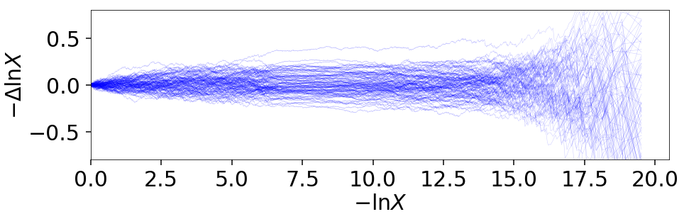
Let’s go through an example using the results from Approximate Evidence Errors. First, let’s examine what the distribution of possible prior volumes looks like:
from dynesty import utils as dyfunc

# plot ln(prior volume) changes
for i in range(100):
    dres_j = dyfunc.jitter_run(dres)
    plt.plot(-dres.logvol, -dres.logvol + dres_j.logvol, color='blue',
             lw=0.5, alpha=0.2)
plt.ylim([-0.8, 0.8])
plt.xlabel(r'$-\ln X$')
plt.ylabel(r'$- \Delta \ln X$')
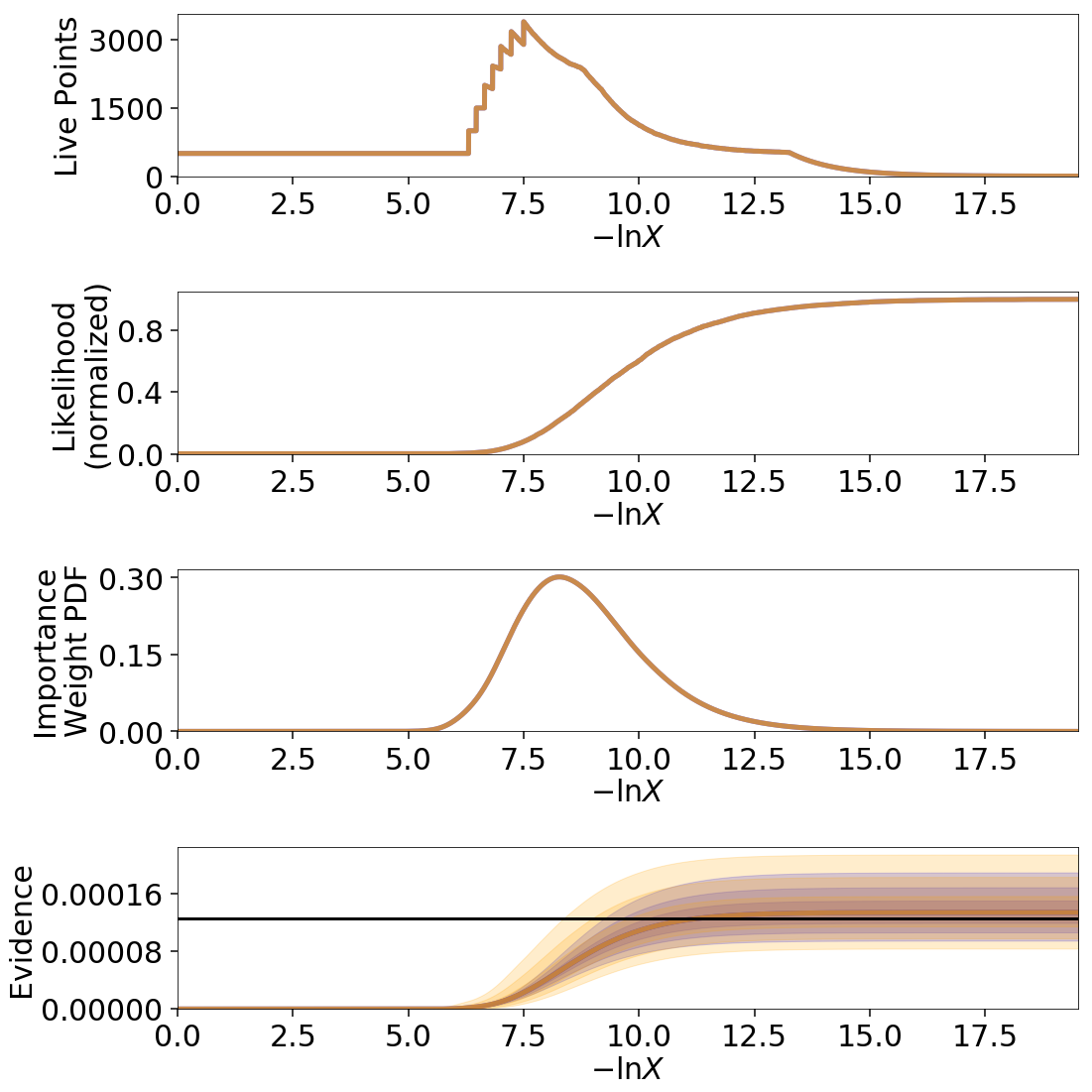
How do these realizations compare with our evidence approximation? We can compare them directly:
import copy

# compute ln(evidence) error
lnzs = np.zeros((100, len(dres.logvol)))
for i in range(100):
    dres_j = dyfunc.jitter_run(dres)
    lnzs[i] = np.interp(-dres.logvol, -dres_j.logvol, dres_j.logz)
lnzerr = np.std(lnzs, axis=0)

# plot comparison
dres_j = copy.deepcopy(dres)
dres_j['logzerr'] = lnzerr
fig, axes = dyplot.runplot(dres, color='blue')
fig, axes = dyplot.runplot(dres_j, color='orange',
                           lnz_truth=lnz_truth, truth_color='black',
                           fig=(fig, axes))
fig.tight_layout()
While the analytic evidence approximations tend to underestimate the error while sampling within the typical set, the final errors are almost identical.
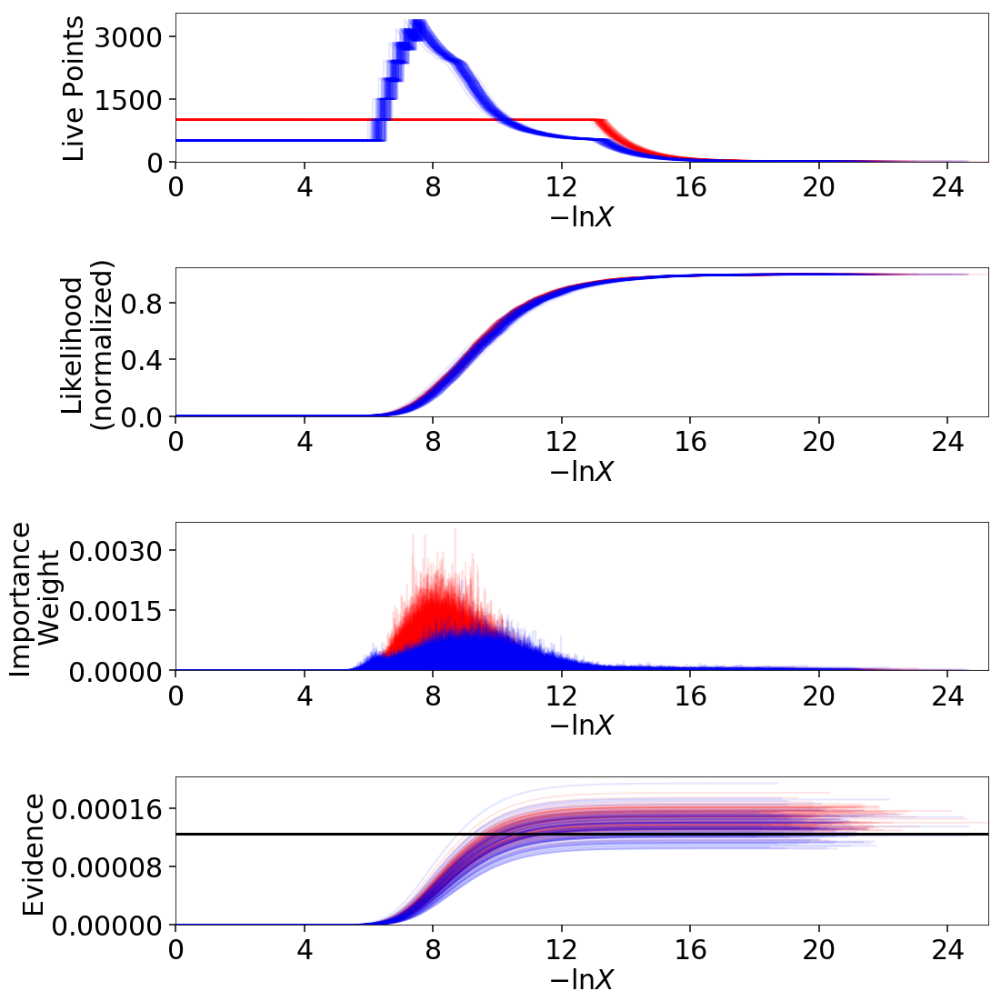
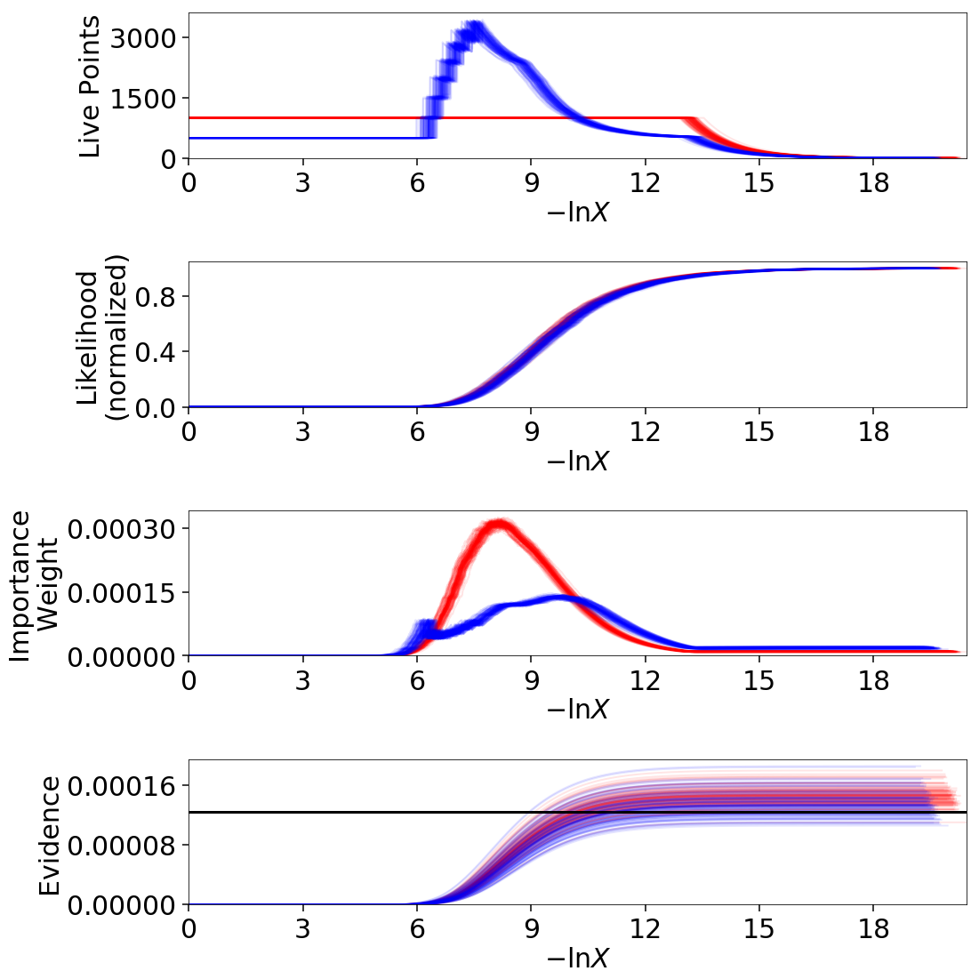
Finally, let’s just plot a number of realizations directly to get a sense of how changes to the prior volumes propagate through to other quantities:
# overplot draws on summary plots
fig, axes = plt.subplots(4, 1, figsize=(16, 16))
for i in range(100):
    res2_j = dyfunc.jitter_run(res2)
    fig, axes = dyplot.runplot(res2_j, color='red',
                               plot_kwargs={'alpha': 0.1, 'linewidth': 2},
                               mark_final_live=False, lnz_error=False,
                               fig=(fig, axes))
for i in range(100):
    dres_j = dyfunc.jitter_run(dres)
    fig, axes = dyplot.runplot(dres_j, color='blue',
                               plot_kwargs={'alpha': 0.1, 'linewidth': 2},
                               mark_final_live=False, lnz_error=False,
                               lnz_truth=lnz_truth, truth_color='black',
                               truth_kwargs={'alpha': 0.1},
                               fig=(fig, axes))
fig.tight_layout()
Sampling Uncertainties
In addition to the statistical uncertainties associated with the unknown prior volumes, Nested Sampling is also subject to sampling uncertainties due to the “path” taken by a particular live point through the prior. This encompasses two different sources of error intrinsic to sampling itself. The first is Monte Carlo noise that arises from probing a continuous distribution using a finite set of samples. The second is path-dependency, where the results depend on the particular paths taken by the set of particles. This affects the results since the number of positions sampled along each path is subject to Poisson noise (see Approximate Evidence Errors); positions can be correlated in some way rather than fully independent draws from the target distribution, subtly violating the sampling assumptions in Nested Sampling.
In other words, although the prior volume \(X_i\) at a given iteration \(i\) might be known exactly, the particular position \(\boldsymbol{\Theta}_i\) on the iso-likelihood contour \(\mathcal{L}_i\) is randomly distributed. This adds some additional noise to our posterior and evidence estimates. This can also complicate things if there are problems with the live point proposals that violate the assumptions described in Nested Sampling.
Unraveling/Merging Runs
One way to interpret Nested Sampling is that it is a scheme that takes a set of ordered likelihoods \(0 < \mathcal{L}_1 < \dots < \mathcal{L}_N\) and associates them with a set of corresponding prior volumes \(1 > X_1 > \dots > X_N > 0\) by means of a number of live points.
One neat property of Nested Sampling is that if we have two Static Nested Sampling runs with \(K_1\) and \(K_2\) live points, respectively, composed of two sets of ordered likelihoods \(0 < \mathcal{L}_{(1)}^{(K_1)} < \dots < \mathcal{L}_{(N)}^{(K_1)}\) and \(0 < \mathcal{L}_{(1)}^{(K_2)} < \dots < \mathcal{L}_{(N)}^{(K_2)}\), the combined set of ordered likelihoods has the same properties as the set of ordered likelihoods associated with a run using \(K_1+K_2\) live points!
This property can be directly extended to merge any combination of \(M\) Static Nested Sampling runs. It can also be applied in reverse to unravel a run with \(K\) live points into \(K\) runs with a single live point. These “strands” form the base unit of a Nested Sampling run.
This “trivially parallelizable” property of Static Nested Sampling can also be directly extended to Dynamic Nested Sampling runs over where strands/batches are added over different likelihood ranges. For instance, combining two runs with \(K_1\) and \(K_2\) live points from \(\mathcal{L}_\min^{(K_1)} < \mathcal{L}_\min^{(K_2)} < \mathcal{L}_\max^{(K_2)} < \mathcal{L}_\max^{(K_1)}\) is equivalent to a Dynamic Nested Sampling run with \(K_1+K_2\) live points between \(\mathcal{L}_\min^{(K_2)} < \mathcal{L}_\max^{(K_2)}\) and \(K_1\) elsewhere.
This process of unraveling/merging Nested Sampling runs can be done using the
unravel_run() and merge_runs()
functions. Both functions work with Static and Dynamic Nested Sampling results,
although some of the provided anciliary quantities are not always valid. Their
usage is straightforward:
res_list = dyfunc.unravel_run(res)  # unravel run into strands
res_merge = dyfunc.merge_runs(res_list)  # merge strands
Note that these functions are mostly included for completeness and are not intended for heavy use in most practical applications.
Bootstrapping Runs
In theory, to properly incorporate these sampling errors we have to marginalize over all possible paths particles can take through the distribution. In practice, however, we can approximate the set of all possible paths using the discrete set of paths taken from the set of \(K\) particles (live points) in a given run. By bootstrap resampling a new set of \(K\) strands (paths) from the current set of \(K\) live points, we are able to construct a new “resampled” run that probes these intrinsic sampling uncertainties. This both allows us to probe Poisson noise in the number of total steps \(N\) as well as the particular path-dependencies of the set of particles.
There is one small caveat to this result. When the number of live points remains constant, there is a symmetry in the information content provided by each strand: since all points are initialized from the prior \(\pi(\boldsymbol{\Theta})\), they provide information on the prior volume \(X\) at a given iteration, allowing for both evidence estimation and posterior inference. Adding live points dynamically, however, can break this symmetry since not all strands are initialized starting from the prior: while these provide relative information useful for posterior inference, they are useless for evidence estimation. Since these two sets of “baseline” and “add-on” strands have qualitatively different properties, we use a stratified bootstrap to preserve their relative contributions to the final set of results.
The resample_run() function implements the bootstrap
resampling approach. It then returns a new Results
dictionary with a new set of samples and associated quantities.
Let’s use the same examples as Jittering Runs to demonstrate it’s usage. First, we will examine how these realizations compare with the original analytic evidence approximation:
# compute ln(evidence) error
lnzs = np.zeros((100, len(dres.logvol)))
for i in range(100):
    dres_r = dyfunc.resample_run(dres)
    lnzs[i] = np.interp(-dres.logvol, -dres_r.logvol, dres_r.logz)
lnzerr = np.std(lnzs, axis=0)

# plot comparison
dres_r = copy.deepcopy(dres)
dres_r['logzerr'] = lnzerr
fig, axes = dyplot.runplot(dres, color='blue')
fig, axes = dyplot.runplot(dres_r, color='orange',
                           lnz_truth=lnz_truth, truth_color='black',
                           fig=(fig, axes))
fig.tight_layout()
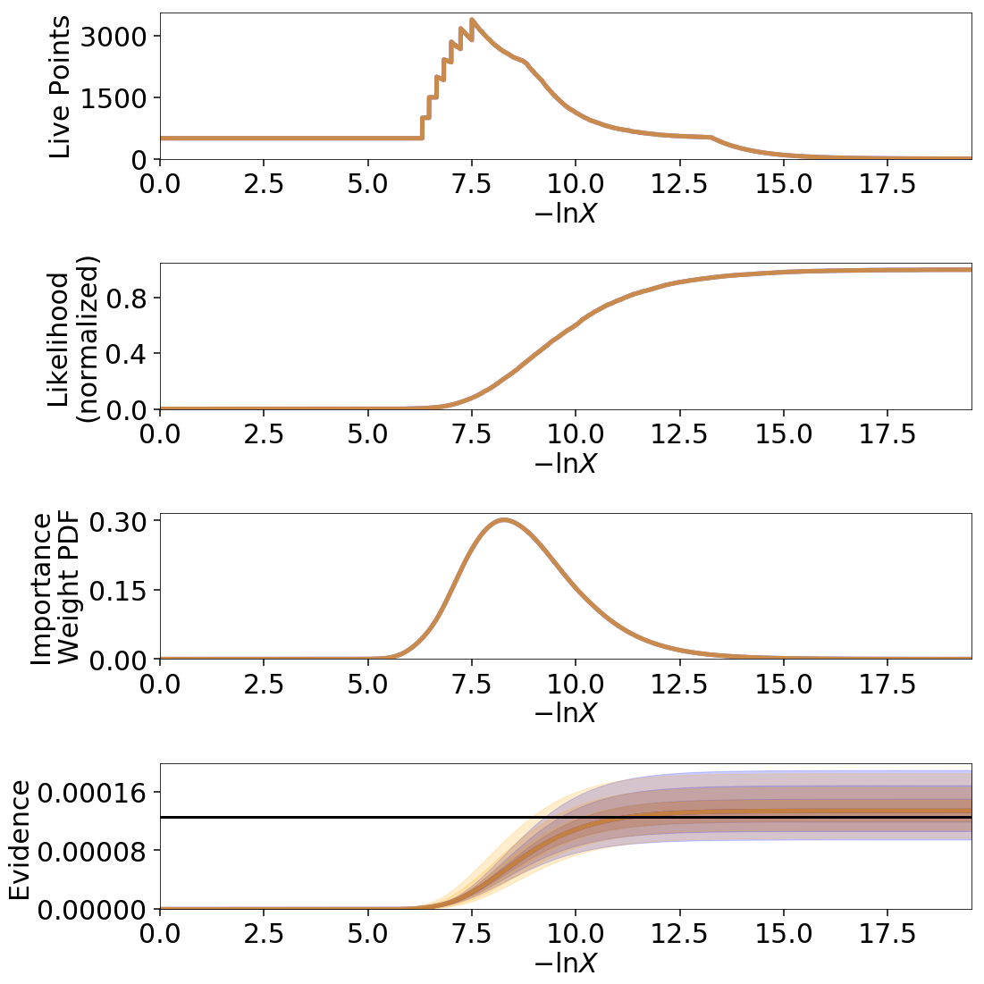
The final errors are again almost identical.
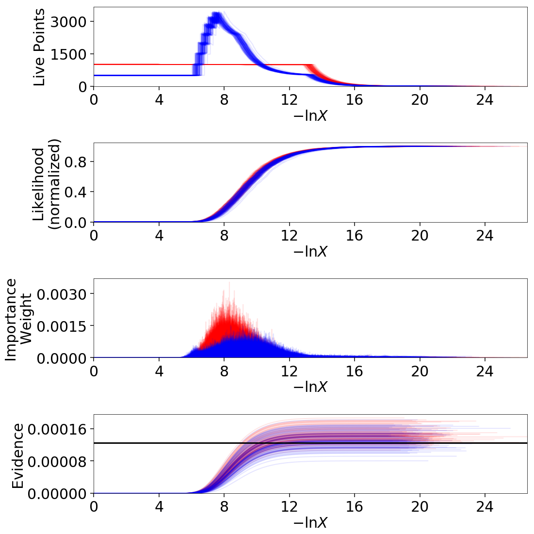
Now let’s just plot a number of realizations directly to get a sense of how our (stratified) bootstrap affects other quantities:
# overplot draws on summary plots
fig, axes = plt.subplots(4, 1, figsize=(16, 16))
for i in range(100):
    res2_r = dyfunc.resample_run(res2)
    fig, axes = dyplot.runplot(res2_r, color='red',
                               plot_kwargs={'alpha': 0.1, 'linewidth': 2},
                               mark_final_live=False, lnz_error=False,
                               fig=(fig, axes))
for i in range(100):
    dres_r = dyfunc.resample_run(dres)
    fig, axes = dyplot.runplot(dres_r, color='blue',
                               plot_kwargs={'alpha': 0.1, 'linewidth': 2},
                               mark_final_live=False, lnz_error=False,
                               lnz_truth=lnz_truth, truth_color='black',
                               truth_kwargs={'alpha': 0.1},
                               fig=(fig, axes))
fig.tight_layout()
Uncertainty Estimates in Practice
Let’s examine the behavior using the same examples as shown in Jittering Runs and Bootstrapping Runs.
# compute ln(evidence) error
lnzs = np.zeros((100, len(dres.logvol)))
for i in range(100):
    dres_s = dyfunc.simulate_run(dres)
    lnzs[i] = np.interp(-dres.logvol, -dres_s.logvol, dres_s.logz)
lnzerr = np.std(lnzs, axis=0)

# plot comparison
dres_s = copy.deepcopy(dres)
dres_s['logzerr'] = lnzerr
fig, axes = dyplot.runplot(dres, color='blue')
fig, axes = dyplot.runplot(dres_s, color='orange',
                           lnz_truth=lnz_truth, truth_color='black',
                           fig=(fig, axes))
fig.tight_layout()
# overplot draws on summary plots
fig, axes = plt.subplots(4, 1, figsize=(16, 16))
for i in range(100):
    res2_s = dyfunc.simulate_run(res2)
    fig, axes = dyplot.runplot(res2_s, color='red',
                               plot_kwargs={'alpha': 0.1, 'linewidth': 2},
                               mark_final_live=False, lnz_error=False,
                               fig=(fig, axes))
for i in range(100):
    dres_s = dyfunc.simulate_run(dres)
    fig, axes = dyplot.runplot(dres_s, color='blue',
                               plot_kwargs={'alpha': 0.1, 'linewidth': 2},
                               mark_final_live=False, lnz_error=False,
                               lnz_truth=lnz_truth, truth_color='black',
                               truth_kwargs={'alpha': 0.1},
                               fig=(fig, axes))
fig.tight_layout()
Validation Against Repeated Runs
As a quick demonstration of usage, we check the fidelity of these results against a set a repeated Nested Sampling runs:
# generate repeat nested sampling runs
Nrepeat = 500
repeat_res = []
dsampler = dynesty.DynamicNestedSampler(loglikelihood, prior_transform,
                                        ndim, bound='single')

for i in range(Nrepeat):
    dsampler.reset()
    dsampler.run_nested(print_progress=False, maxiter=5000, use_stop=False)
    repeat_res.append(dsampler.results)
# establish our comparison run
dsampler.reset()
dsampler.run_nested(print_progress=False, maxiter=5000, use_stop=False)
r = dsampler.results

# generate jittered runs
sim_res = []
for i in range(Nrepeat):
    sim_res.append(dyfunc.jitter_run(r))

# generate resampled runs
rsamp_res = []
for i in range(Nrepeat):
    rsamp_res.append(dyfunc.resample_run(r))
As an initial test, we can compare the estimated \(\ln \hat{\mathcal{Z}}\) from each set of runs:
# compare evidence estimates

# analytic first-order approximation
lnz_mean, lnz_std = r.logz[-1], r.logzerr[-1]
print('Approx.:     {:6.3f} +/- {:6.3f}'.format(lnz_mean, lnz_std))

# jittered draws
lnz_arr = [results.logz[-1] for results in jitter_res]
lnz_mean, lnz_std = np.mean(lnz_arr), np.std(lnz_arr)
print('Sim.:        {:6.3f} +/- {:6.3f}'.format(lnz_mean, lnz_std))

# resampled draws
lnz_arr = [results.logz[-1] for results in rsamp_res]
lnz_mean, lnz_std = np.mean(lnz_arr), np.std(lnz_arr)
print('Resamp.:     {:6.3f} +/- {:6.3f}'.format(lnz_mean, lnz_std))

# repeated runs
lnz_arr = [results.logz[-1] for results in repeat_res]
lnz_mean, lnz_std = np.mean(lnz_arr), np.std(lnz_arr)
print('Repeat: {:6.3f} +/- {:6.3f}'.format(lnz_mean, lnz_std))
Out:
Approx.:     -8.670 +/-  0.207
Sim.:        -8.696 +/-  0.192
Resamp.:     -8.676 +/-  0.180
Repeat:      -8.912 +/-  0.211
We find the approximate, simulated, and resampled uncertainties show relatively good agreement.
We can also compare the first and second moments of the posterior:
# compare posterior first moments

# jittered draws
x_arr = np.array([dyfunc.mean_and_cov(results.samples,
                  weights=np.exp(results.logwt))[0]
                  for results in jitter_res])
x_mean = np.round(np.mean(x_arr, axis=0), 3)
x_std = np.round(np.std(x_arr, axis=0), 3)
print('Sim.:        {0} +/- {1}'.format(x_mean, x_std))

# resampled draws
x_arr = np.array([dyfunc.mean_and_cov(results.samples,
                  weights=np.exp(results.logwt))[0]
                  for results in rsamp_res])
x_mean = np.round(np.mean(x_arr, axis=0), 3)
x_std = np.round(np.std(x_arr, axis=0), 3)
print('Resamp.:     {0} +/- {1}'.format(x_mean, x_std))

# repeated runs
x_arr = np.array([dyfunc.mean_and_cov(results.samples,
                  weights=np.exp(results.logwt))[0]
                  for results in repeat_res])
x_mean = np.round(np.mean(x_arr, axis=0), 3)
x_std = np.round(np.std(x_arr, axis=0), 3)
print('Rep. (mean): {0} +/- {1}'.format(x_mean, x_std))
Out:
Sim.:        [-0.022 -0.022 -0.021] +/- [0.016 0.016 0.016]
Resamp.:     [-0.023 -0.023 -0.022] +/- [0.016 0.017 0.017]
Repeat:      [ 0.002  0.002  0.002] +/- [0.016 0.016 0.016]
# compare posterior second (diagonal) moments

# jittered draws
x_arr = np.array([dyfunc.mean_and_cov(results.samples,
                  weights=np.exp(results.logwt))[1]
                  for results in jitter_res])
x_arr = [np.diag(x) for x in x_arr]
x_mean = np.round(np.mean(x_arr, axis=0), 3)
x_std = np.round(np.std(x_arr, axis=0), 3)
print('Sim.:        {0} +/- {1}'.format(x_mean, x_std))

# resampled draws
x_arr = np.array([dyfunc.mean_and_cov(results.samples,
                  weights=np.exp(results.logwt))[1]
                  for results in rsamp_res])
x_arr = [np.diag(x) for x in x_arr]
x_mean = np.round(np.mean(x_arr, axis=0), 3)
x_std = np.round(np.std(x_arr, axis=0), 3)
print('Resamp.:     {0} +/- {1}'.format(x_mean, x_std))

# repeated runs
x_arr = np.array([dyfunc.mean_and_cov(results.samples,
                  weights=np.exp(results.logwt))[1]
                  for results in repeat_res])
x_arr = [np.diag(x) for x in x_arr]
x_mean = np.round(np.mean(x_arr, axis=0), 3)
x_std = np.round(np.std(x_arr, axis=0), 3)
print('Rep. (mean): {0} +/- {1}'.format(x_mean, x_std))
Out:
Sim.:        [1.041 1.038 1.046] +/- [0.026 0.026 0.026]
Resamp.:     [1.039 1.035 1.044] +/- [0.026 0.026 0.027]
Repeat:      [0.994 0.994 0.993] +/- [0.026 0.026 0.026]
Our simulated and resampled uncertainties seem to do an excellent job of capturing the intrinsic uncertainties in both the mean and the standard deviation here.
Posterior Uncertainties
As discussed in How Many Samples are Enough?, it can be difficult to determine how many samples are needed to guarantee the posterior density estimate \(\hat{P}(\boldsymbol{\Theta})\) constructed from the set of samples \(\left\lbrace \boldsymbol{\Theta}_1, \dots, \boldsymbol{\Theta}_N \right\rbrace\) is a “good” approximation to the true posterior density \(P(\boldsymbol{\Theta})\). One way of getting a handle on this is to measure the “difference” between the two distributions using the KL divergence:
Since we do not know \(P(\boldsymbol{\Theta})\), we can substitute \(\hat{P} \rightarrow \hat{P}^\prime\) and \(P \rightarrow \hat{P}\) to construct an empirical estimate of this quantity based on realizations of \(\hat{P}(\boldsymbol{\Theta})\):
KL divergences between (realizations of) Nested Sampling runs can be computed
in dynesty using the
kld_error() functions.
Let’s examine the results from the Static Nested
Sampling run used above to get a sense of what these look like:
# compute KL divergences
klds = []
for i in range(Nrepeat):
    kld = dyfunc.kld_error(res2, error='jitter')
    klds.append(kld)

# plot (cumulative) KL divergences
plt.figure(figsize=(12, 5))
for kld in klds:
    plt.plot(kld, color='red', alpha=0.15)
plt.xlabel('Iteration')
plt.ylabel('KL Divergence');
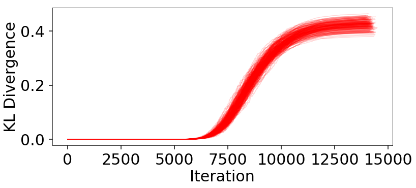
The behavior appears qualitatively similar to our evidence results, since the majority of the KL divergence is coming from integrating over the bulk of the posterior mass in the typical set. The variation in these results are plotted below:
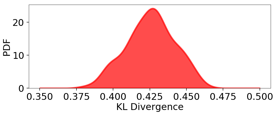
from scipy.stats import gaussian_kde

# compute KLD kernel density estimate
kl_div = [kld[-1] for kld in klds]
kde = gaussian_kde(kl_div)

# plot results
plt.figure(figsize=(10, 4))
x = np.linspace(0.35, 0.5, 1000)
plt.fill_between(x, kde.pdf(x), color='red', alpha=0.7, lw=5)
plt.ylim([0., None])
plt.xlabel('KL Divergence')
plt.ylabel('PDF')

# summarize results
kl_div_mean, kl_div_std = np.mean(kl_div), np.std(kl_div)
print('Mean:   {:6.3f}'.format(kl_div_mean))
print('Std:    {:6.3f}'.format(kl_div_std))
print('Std(%): {:6.3f}'.format(kl_div_std / kl_div_mean * 100.))
Out:
Mean:    0.425
Std:     0.016
Std(%):  3.833
Our Dynamic Nested Sampling run contains the same number of samples but preferentially places them around the typical set to improve posterior estimation. The corresponding results are shown below for comparison:
klds2 = []
for i in range(Nrepeat):
    kld2 = dyfunc.kld_error(dres)
    klds2.append(kld2)

# compute KLD kernel density estimate
kl_div2 = [kld2[-1] for kld2 in klds2]
kde2 = gaussian_kde(kl_div2)

# plot results
plt.figure(figsize=(14, 5))
plt.fill_between(x, kde.pdf(x), color='red', alpha=0.7, lw=5)
plt.fill_between(x, kde2.pdf(x), color='blue', alpha=0.7, lw=5)
plt.ylim([0., None])
plt.xlabel('KL Divergence')
plt.ylabel('PDF')

# summarize results
kl_div2_mean, kl_div2_std = np.mean(kl_div2), np.std(kl_div2)
print('Mean:   {:6.3f}'.format(kl_div2_mean))
print('Std:    {:6.3f}'.format(kl_div2_std))
print('Std(%): {:6.3f}'.format(kl_div2_std / kl_div2_mean * 100.))
Out:
Mean:    0.423
Std:     0.012
Std(%):  2.909
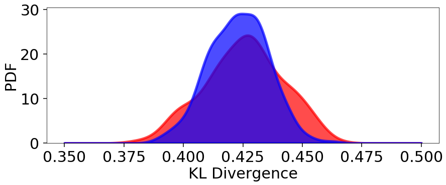
We see that although the mean KL divergence is similar, the fractional variation around the mean is smaller.