Getting Started

Prior Transforms

The prior transform function is used to implicitly specify the Bayesian prior \(\pi(\boldsymbol{\Theta})\) for Nested Sampling. It functions as a transformation from a space where variables are i.i.d. within the \(D\)-dimensional unit cube (i.e. uniformly distributed from 0 to 1) to the parameter space of interest. For independent parameters, this would be the product of the inverse cumulative distribution function (CDF) (also known as the “percent point function” or “quantile function”) associated with each parameter.

It is crucial to note that increasing the size of the prior directly impacts the amount of time needed to integrate over the posterior. We highlight some examples of prior transforms below.

Example: Uniform Priors

Suppose we want our prior to be Uniform from [-10, 10) for all variables:

\[\begin{split}p(x) \propto \left\{ \begin{array}{ll} 1 \quad -10 \le x < 10\\ 0 \quad {\rm otherwise} \end{array} \right.\end{split}\]

The prior transform for this distribution would be:

def prior_transform(u):
    """Transforms the uniform random variable `u ~ Unif[0., 1.)`
    to the parameter of interest `x ~ Unif[-10., 10.)`."""

    x = 2. * u - 1.  # scale and shift to [-1., 1.)
    x *= 10.  # scale to [-10., 10.)

    return x

Example: Non-uniform priors

Suppose we instead have a more complicated prior in 5 variables. The first 2 are drawn from a bivariate Normal distribution, the third is drawn from a Beta distribution, the fourth from a Gamma distribution, and the fifth from a truncated normal distribution. To handle more complicated functions like these, we can use the built-in functions in scipy.stats, which include a percent point function (ppf) that is analogous to our prior transform. Using those, our above examples would look like:

def prior_transform(u):
    """Transforms the uniform random variables `u ~ Unif[0., 1.)`
    to the parameters of interest."""

    x = np.array(u)  # copy u

    # Bivariate Normal
    t = scipy.stats.norm.ppf(u[0:2])  # convert to standard normal
    Csqrt = np.array([[2., 1.],
                      [1., 2.]])  # C^1/2 for C=((5, 4), (4, 5))
    x[0:2] = np.dot(Csqrt, t)  # correlate with appropriate covariance
    mu = np.array([5., 2.])  # mean
    x[0:2] += mu  # add mean

    # Beta
    a, b = 2.31, 0.627  # shape parameters
    x[2] = scipy.stats.beta.ppf(u[2], a, b)

    # Gamma
    alpha = 5.  # shape parameter
    x[3] = scipy.stats.gamma.ppf(u[3], alpha)

    # Truncated Normal
    m, s = 5, 2  # mean and standard deviation
    low, high = 2., 10.  # lower and upper bounds
    low_n, high_n = (low - m) / s, (high - m) / s  # standardize
    x[4] = scipy.stats.truncnorm.ppf(u[4], low_n, high_n, loc=m, scale=s)

    return x

Example: Conditional priors

This procedure can be generalized to construct priors that only can be expressed in conditional form. As an example, let’s assume we have a three-parameter model where the prior for the third parameter depends on the values for the first two. This might be the case in, e.g., a hierarchical model where the prior over c is a Normal distribution whose mean m and standard deviation s are determined by a corresponding “hyper-prior”. We can easily set up a prior transform for this model by just going through the variables in order. This would look like:

def prior_transform(u):
    """Transforms the uniform random variables `u ~ Unif[0., 1.)`
    to the parameters of interest."""

    x = np.array(u)  # copy u

    # Mean hyper-prior
    mu, sigma = 5., 1.  # mean, standard deviation
    x[0] = scipy.stats.norm.ppf(u[0], loc=mu, scale=sigma)

    # Standard deviation hyper-prior
    x[1] = 10. ** (u[1] * 2. - 1.)  # log10(std) ~ Uniform[-1, 1]

    # Prior
    x[2] = scipy.stats.norm.ppf(u[2], loc=x[0], scale=x[1])

    return x

More complicated dependencies can be constructed using similar approaches.

Nested Sampling with dynesty

To give a concrete example of running dynesty on a real problem, let’s return to the simple 3-D multivariate normal likelihood and uniform prior from [-10, 10) used in Crash Course to define the loglikelihood() and prior_transform() functions:

import numpy as np

# Define the dimensionality of our problem.
ndim = 3

# Define our 3-D correlated multivariate normal log-likelihood.
C = np.identity(ndim)
C[C==0] = 0.95
Cinv = linalg.inv(C)
lnorm = -0.5 * (np.log(2 * np.pi) * ndim +
                np.log(np.linalg.det(C)))

def loglike(x):
    return -0.5 * np.dot(x, np.dot(Cinv, x)) + lnorm

# Define our uniform prior via the prior transform.
def ptform(u):
    return 20. * u - 10.

Initialization

Nested Sampling in dynesty is done via a particular sampler object that is initialized from the Top-Level Interface. To start, let’s use NestedSampler() to initialize a particular sampler from nestedsamplers. There are only 3 required arguments: a log-likelihood function (loglike), a prior transform function (ptform), and the number of dimensions taken by the loglikelihood (ndim).

Using the functions above, we can initialize our sampler using:

from dynesty import NestedSampler

# initialize our nested sampler
sampler = NestedSampler(loglike, ptform, ndim)

See Top-Level Interface for more details on the API, Examples for more examples of usage, and FAQ for some additional advice. Here we’ll go over just the basics.

Live Points

Similar to ensemble sampling methods such as emcee, the behavior of Nested Sampling can also be sensitive to the number of live points used. Increasing the number of live points leads to smaller changes in the prior volume \(\ln X\) over time. This improves the effective resolution while simultaneously increasing the runtime.

In addition, the number of live points can also affect the stability of our Bounding Options. By default, dynesty inflates the size of the chosen bounds by an enlargement factor to ensure they effectively bound the iso-likelihood contours. These bounds become more robust the more live points are used, leading to more efficient proposals.

It is important to note that running with too few live points can lead to mode “die off”. When there are multiple modes with live points distributed between them, live points can randomly “jump” between them at any given iteration. If there are only a handful of live points at a particular mode, it is possible that, entirely by chance, all of them could transfer completely to the other mode even as both remain equally likely, leading it to “die off” and likely never be located again. As a rule-of-thumb, you should allocate around 50 live points per possible mode to guard against this.

The number of live points can be specified upon initialization via the nlive argument. For example, if we want to run with 1000 live points rather than the default 250, we would use:

NestedSampler(loglike, ptform, ndim, nlive=1500)

Bounding Options

dynesty supports a number of options for bounding the target distribution:

no bound ('none'), i.e. sampling from the entire unit cube,
a single bounding ellipsoid ('single'),
multiple (possibly overlapping) bounding ellipsoids ('multi'),
overlapping balls centered on each live point ('balls'), and
overlapping cubes centered on each live point ('cubes').

By default, dynesty uses multi-ellipsoidal decomposition ('multi'), which often is flexible enough to capture the complexity of many likelihood distributions while simple enough to quickly and efficiently generate new samples. For more complex distributions, overlapping balls ('balls') or cubes ('cubes') can generate more flexible bounding distributions but come with significantly more overhead that can be less efficient at generating samples. For simpler distributions, a single ellipsoid ('single') is often sufficient. Sampling directly from the unit cube ('none') is extremely inefficient but is a useful option to verify your results and look for possible biases. It otherwise should only be used if the log-likelihood is trivial to compute.

Specifying the particular bounding distribution can be done upon initialization via the bound argument. If we wanted to sample using overlapping balls rather than multiple bounding ellipsoids, for instance, we would use:

NestedSampler(loglike, ptform, ndim, nlive=1500, bound='balls')

As mentioned in Live Points, bounding distributions in dynesty are enlarged in an attempt to conservatively encompass the iso-likelihood contour associated with each dead point. The default behavior increases the volume by 25%, although this can also be done in real-time using bootstrapping methods (this procedure can lead to some instability in the size of the bounds if fewer than the optimal number of live points are being used; see the FAQ for additional details). The volume enlargement factor or the number of bootstrap realizations used can be specified using the enlarge and bootstrap arguments.

Additional information on the bounding objects can be found under Bounding and in Examples.

To avoid excessive overhead spent constructing bounding distributions, dynesty only updates bounding distributions after a fixed number of likelihood calls specified by the update_interval argument. Larger values generally decrease the sampling efficiency but can improve overall performance. This value by default is set to different values for different sampling methods (see the API for additional details), but if we wanted to instead use a particular value we could just specify that via:

NestedSampler(loglike, ptform, ndim, nlive=1500, bound='balls',
              bootstrap=50, update_interval=1.2)

Passing a float like 1.2 sets the update interval to be after round(1.2 * nlive) functional calls so that it scales based on the number of live points (and thus the speed at which we expect to traverse the prior volume). If we’d like to specific the number of function calls directly, however, we can instead pass an integer:

NestedSampler(loglike, ptform, ndim, nlive=1500, bound='balls',
              bootstrap=50, update_interval=600)

This now specifies that we will update our bounds after 600 function calls.

See Top-Level Interface for more information.

Sampling Options

dynesty also supports several different sampling methods conditioned on the provided bounds which can be passed via the sample argument:

uniform sampling ('unif'),
random walks away from a current live point ('rwalk'),
multivariate slice sampling away from a current live point ('slice'),
random slice sampling away from a current live point ('rslice'), and
“Hamiltonian” slice sampling away from a current live point ('hslice').

In addition, dynesty also supports passing custom callable functions to the sample argument, provided they follow the same format as the default sampling functions defined here. These can also be accompanied by custom “update functions” that try to adaptively scale proposals to ensure better overall sampling efficiency. See here for examples of some of the functions that are associated with the default sampling methods described above.

By default, dynesty automatically picks a sampling method based on the dimensionality of the problem via the 'auto' argument, which uses the following logic:

If \(D < 10\), 'unif' is chosen since uniform proposals can be quite efficient in low dimensions.
If \(10 \leq D \geq 20\), 'rwalk' is chosen since random walks are more robust to underestimated bounding distributions in higher dimensions,
If \(D > 20\) and a gradient is not provided, 'rslice' is chosen since non-rejection sampling methods scale in polynomial (rather than exponential) time as the dimensionality increases.
If \(D > 20\) and a gradient is provided, 'hslice' is chosen to take advantage of Hamiltonian dynamics, which scale better than 'rslice' as the dimensionality increases.

Note that 'hslice', while using gradients, is substantially less efficient (and in general less reliable) than other gradient-based approaches such as Hamiltonian Monte Carlo. As such, use them at your own risk.

One benefit to using random walks or slice sampling is that they require many fewer live points to adapt to structure in higher dimensions (since they only sample conditioned on the bounds, rather than within them). They also do not require any sort of bootstrap-style corrections since they contain built-in methods to tune their step sizes. This, however, does not mean that they are immune to issues that arise when running with fewer live points such as mode “die-off” (see Live Points).

Following the example above, let’s say we wanted to combine the flexibility of multiple bounding ellipsoids and slice sampling. This might look something like:

NestedSampler(loglike, ptform, ndim, bound='multi', sample='slice')

See Top-Level Interface for additional information.

Early-Time Behavior

dynesty tries to avoid constructing bounding distributions early in the run to avoid issues where the bounds can significantly exceed the unit cube. For instance, in most cases the bounding distribution of the initial set of points by construction will exceed the bounds of the unit cube when enlarge > 1. This can lead to a variety of problems associated with each method, especially in higher dimensions (since volume scales as \(\propto r^D\)).

To avoid this behavior, dynesty deliberately delays the first bounding update until at least 2 * nlive function calls have been made and the efficiency has fallen to 10%. This generally assumes that the overall efficiency will be below 10%, which is the case for almost all sampling methods (see below). If we wanted to adjust this behavior so that we construct our first bounding distributions much earlier, we could do so by passing some parameters using the first_update argument:

NestedSampler(loglike, ptform, ndim, nlive=1500, bound='balls',
              first_update={'min_ncall': 100, 'min_eff': 50.})

This will now trigger an update when 100 log-likelihood function calls have been made and the efficiency drops below 50%.

Special Boundary Conditions

By default, dynesty assumes that all parameters have hard bounds. In other words, if for some reason you propose outside of the unit cube that defines the prior (see Prior Transforms), that point is automatically rejected and a new one is proposed instead. This is the desired behavior for most problems, since individual parameters are often either defined everywhere (i.e. from negative infinity to infinity) or over a finite range (e.g., from \(10\) to \(25\)).

Specific problems, however, may have parameters that behave differently. In particular, dynesty supports both reflective and periodic boundary conditions. The former can arise when parameters are ratios (where \(1/2\) and \(2/1\) may be equivalent) or angles (since 90 degrees and 450 degrees are often equivalent). Imposing these specific boundary conditions on relevant parameters can help improve the overall sampling efficiency, especially when solutions end up near the bounds (e.g., at \(0\) or \(2\pi\) for phases). These can be enabled by just specifying the indices of the relevant parameters, as shown below:

NestedSampler(loglike, ptform, ndim, nlive=1000, bound='cubes',
              periodic=[0, 2], reflective=[1, 5])

Parallelization

If you want to run computations in parallel, dynesty can use a user-defined pool to execute a variety of internal operations in “parallel” rather than in serial. This can be done by passing the pool object to the sampler upon initialization:

# initialize sampler with pool
sampler = NestedSampler(loglike, ptform, ndim, pool=pool)

By default, dynesty tries to grab the size of the pool from the pool.size attribute of the pool. If this is not defined, the number of function evaluations to execute in parallel can be set manually using the queue_size argument:

# initialize sampler with pool with pre-defined queue
sampler = NestedSampler(loglike, ptform, ndim, pool=pool, queue_size=8)

There is no reason to set queue_size to anything other then the number of parallel processes in the pool.

Parallel operations in dynesty are done by simply swapping in the pool.map function over the default map function when making likelihood calls. Note that this is a synchronous function call, which requires that all members of the pool have completed their respective tasks before receiving the pool’s output. The call time for functions is therefore limited by the slowest-performing member of the pool.

The reason why “parallel” is written in quotes above is that while function evaluations can be made in parallel, live point proposals must be done serially in order to avoid breaking the statistical properties of Nested Sampling. Assuming we are using \(M\) processes with \(K\) live points, this leads to sub-linear speed improvements \(S\) of the form (Handley et al. 2015):

\[S(M, K) = K \ln \left(1 + \frac{M}{K}\right)\]

This scales pretty linearly with the number of processes till the number of parallel processes is equal or larger than the number of live-points.

Depending on where the bottleneck of the computation lies, the provided pool can be disabled during certain function evaluations (e.g., when initializing points) using the use_pool argument:

# initialize sampler with pool with pre-defined queue
sampler = NestedSampler(loglike, ptform, ndim,
                        nlive=2000, bound='single', sample='rwalk',
                        pool=pool, queue_size=16,
                        use_pool={'prior_transform': False})

See Pool/Parallelization Questions on the FAQ page for additional troubleshooting tips.

Note that, as discussed in Combining Runs, it is actually possible to combine multiple independent Nested Sampling runs into a single run, giving users an option as to whether they want to parallelize dynesty during runtime (using a user-provided pool) or after runtime (by merging the runs together).

Dynesty multiprocessing pool

If you are running multiprocessing on a single machine, probably the easiest way of parallelizing is using a dynesty provided pool (which is a thin wrapper around python’s multiprocessing pool):

with Pool(10, loglike, ptform) as pool:
    sampler = NestedSampler(pool.loglikehood, pool.prior_transform,
                            ndim, pool = pool)
    sampler.run_nested()

Note that we provide the likelihood function and prior transforms when we initialize the pool. When we run dynesty we provide the loglikelihood and prior transforms from the pool. This approach minimizes the overhead from picking function repeatedly.

Note that if your likelihood and/or prior transform take additional arguments, it is usually better specify them when initializing the pool. That is particularly convenient if those arguments are very large as you do not suffer from repeated pickling of those arguments:

with Pool(10, loglike, ptform, logl_args=loglike_args,
                                logl_kwargs=logl_kwargs,
                                ptform_args=ptform_args,
                                ptform_kwargs=ptform_kwargs) as pool:
    sampler = NestedSampler(pool.loglikehood, pool.prior_transform,
                            ndim, pool = pool)
    sampler.run_nested()

If you specified them when creating the pool, you do not need to provide them again to the sampler.

If you specify logl_args, and ptform_args when creating the Pool AND in the sampler those will be concatenated.

Running Internally

Sampling from our target distribution can be done using the run_nested() function in the provided sampler:

sampler.run_nested()

Sampling will continue until specified stopping criteria are reached, and the current state of the sampler is by default output to stderr in real time. The stopping criteria can be any combination of:

a fixed number of iterations (maxiter),
a fixed number of likelihood calls (maxcall),
a maximum log-likelihood (logl_max),
a specified \(\Delta \ln \hat{\mathcal{Z}}_i\) tolerance (dlogz), and
a specified Effective Sample Size (ESS) (n_effective).

For instance, running one of the examples above would produce output like:

Out:

iter: 12521 | +1500 | bound: 7 | nc: 1 | ncall: 66884 | eff(%): 20.963 |
loglstar:   -inf < -0.301 <    inf | logz: -8.960 +/-  0.082 |
dlogz:  0.001 >  1.509

From left to right, this records: the current iteration (plus the number of live points added after stopping), the current bound being used, the number of log-likelihood calls made before accepting the last sample, the total number of log-likelihood calls, the overall sampling efficiency, the current log-likelihood bounds (-inf and inf because we began sampling from the prior and didn’t declare a logl_max), the current estimated evidence, and the remaining dlogz relative to the stopping criterion.

By default, the stopping criteria are optimized for evidence estimation, with posteriors treated as a nice byproduct. We can modify this by passing in something like:

sampler.run_nested(dlogz=0.5, maxiter=10000, maxcall=50000)

Since sampling is done through the sampler objects, users can also continue to add new samples based on where they left off. This is as easy as:

# initialize our sampler
sampler = NestedSampler(loglike, ptform, ndim, nlive=1000)

# start our run
sampler.run_nested(dlogz=0.5)
res1 = sampler.results

# (possibly) add more samples
sampler.run_nested(maxcall=10000)
res2 = sampler.results

# (possibly) add more samples again
sampler.run_nested(dlogz=0.01)
res3 = sampler.results

Checkpointing

While running the sampler using run_nested() interface it is possible to check-point (or save) the state of the sampler into a file at regular intervals. This file can then be used to restart/resume the sampling:

# initialize our sampler
sampler = NestedSampler(loglike, ptform, ndim, nlive=1000)
# run the sampler with checkpointing
sampler.run_nested(checkpoint_file='dynesty.save')

You can then restore it now and resume sampling:

# restore our sampler
sampler = NestedSampler.restore('dynesty.save')
# resume
sampler.run_nested(resume=True)

If you used the pool in the sampler and you want to use the pool after restoring, you need to specify it when restoring:

mypool = multiprocessing.Pool(6)
# restore the sampler
sampler = NestedSampler.restore('dynesty.save', pool =mypool)
# resume
sampler.run_nested(resume=True)

The checkpointing may be helpful if you are running dynesty on HPC with a queue system that has a limit on a wall-time that your jobs can run. There is a however an important reminder that should NOT use checkpointing for persistence. I.e. if you want to save the results of the sampling, you should save samples, weights or the results object, rather than the whole nested sampling object (as checkpointing does). The reason for this is that the checkpoint files are not guaranteed to be compatible between dynesty versions (even minor ones).

Saving auxiliary information from log-likelihood function

Occasionally it is useful to save the information computed by the likelihood function, such as various derived quantities. This information can be easily saved by dynesty together with the samples. To do that you need to use the blob option of NestedSampler and DynamicNestedSampler:

def loglike(x):
    logl = -0.5 * np.sum(x**2)
    blob = np.zeros(3)
    blob[0] = x[0]
    blob[1] = x[1]**2
    blob[2] = logl+x[2]
    # here the logl function return the logl and a numpy array
    return logl, blob
# initialize our sampler
sampler = NestedSampler(loglike, ptform, ndim, nlive=100, blob=True)
# run the sampler with checkpointing
sampler.run_nested()
results = sampler.results
aux_blob = results['blob']
# This variable will contain auxiliary blobs associated with samples

The numpy blob can return arbitrary 1D numpy arrays. The can be record arrays as well. The only requirement is that the shape/dtype is exactly the same between the log-likelihood function calls.

Running Externally

Similar to emcee, sampler objects in dynesty can also be run externally as a generator via the sample() function. This might look something like:

# The main nested sampling loop.
for it, res in enumerate(sampler.sample(dlogz=0.5)):
    pass

# Adding the final set of live points.
for it_final, res in enumerate(sampler.add_live_points()):
    pass

as opposed to:

# The main nested sampling loop.
sampler.run_nested(dlogz=0.5, add_live=False)

# Adding the final set of live points.
sampler.add_final_live()

This can be extremely useful if you would like to manipulate the results in real-time, generate plots, save intermediate outputs, etc.

Combining Runs

Nested sampling is “trivially parallelizable”, which makes it really straightforward to combine the results from multiple independent runs. dynesty contains built-in utilities for combining results from separate runs into a single run with improved posterior/evidence estimates. This can be extremely useful if, for instance, you have performed multiple independent analyses over the course of a project that you would like to combine, or if you want to add additional samples to a preliminary analysis (but don’t have the sampler currently loaded in memory).

dynesty makes this process relatively straightforward. An example is shown below:

from dynesty import utils as dyfunc

# Create several independent nested sampling runs.
sampler = NestedSampler(loglike, ptform, ndim)
rlist = []
for i in range(10):
    sampler.run_nested()
    rlist.append(sampler.results)
    sampler.reset()

# Merge into a single run.
results = dyfunc.merge_runs(rlist)

This process works with Dynamic Nested Sampling as well. See Unraveling/Merging Runs for additional details.

Sampling with Gradients

As mentioned in Sampling Options, dynesty can utilize log-likelihood gradients \(\nabla \ln \mathcal{L}\) by proposing new samples using Hamiltonian dynamics (often referred to as reflective slice sampling). However, because sampling in dynesty occurs on the unit cube (\(\mathbf{u}\)) rather than in the target space of our original variables (\(\mathbf{x}\)), these gradients have to be defined with respect to \(\mathbf{u}\) rather than \(\mathbf{x}\) even though they are evaluated at \(\mathbf{x}\). This requires computing the Jacobian matrix \(\mathbf{J}\) from \(\mathbf{x}\) to \(\mathbf{u}\).

While this Jacobian might seem difficult to derive, it can be shown that given independent priors on each parameter

\[\pi(\mathbf{x}) = \prod_i \pi_i(x_i)\]

where \(\pi_i(x_i)\) is the prior for the i-th parameter \(x_i\) that the Jacobian is diagonal where each diagonal element is simply

\[J_ii = 1 / \pi_i(x_i)\]

By default, dynesty assumes that any gradient you pass in already has the appropriate Jacobian applied. If not, you can tell dynesty to numerically estimate the Jacobian by setting compute_jac=True.

For the simple 3-D multivariate normal likelihood and uniform prior from [-10, 10) used in Crash Course, sampling with gradients would look something like:

import numpy as np
import dynesty

# Define the dimensionality of our problem.
ndim = 3

# Define our 3-D correlated multivariate normal log-likelihood.
C = np.identity(ndim)
C[C==0] = 0.95
Cinv = linalg.inv(C)
lnorm = -0.5 * (np.log(2 * np.pi) * ndim +
                np.log(np.linalg.det(C)))

def loglike(x):
    return -0.5 * np.dot(x, np.dot(Cinv, x)) + lnorm

# Define our uniform prior via the prior transform.
def ptform(u):
    return 20. * u - 10.

# Define our gradient with and without the Jacobian applied.
def grad_x(x):
    return -np.dot(Cinv, x)  # without Jacobian

def grad_u(x):
    return -np.dot(Cinv, x) * 20.  # with Jacobian for uniform [-10, 10)

# Sample with `grad_u` (including Jacobian).
sampler = dynesty.NestedSampler(loglike, ptform, ndim, sample='hslice',
                                gradient=grad_u)
sampler.run_nested()
results_with_jac = sampler.results

# Sample with `grad_x` (compute Jacobian numerically).
sampler = dynesty.NestedSampler(loglike, ptform, ndim, sample='hslice',
                                gradient=grad_x, compute_jac=True)
sampler.run_nested()
results_without_jac = sampler.results

For other independent priors discussed in Prior Transforms, we can use the built-in functions in scipy.stats, which include a probability density function (pdf) that is exactly our desired \(\pi_i(v_i)\) function. These then enable us to compute and apply the (diagonal) Jacobian matrix directly. In more complex cases such as the simple hierarchical model in Example: Conditional priors, however, we may need to resort to estimating the Jacobian numerically to deal with the expected off-diagonal terms.

Results

Sampling results can be accessed through the results property and are returned as a (modified) dictionary:

results = sampler.results

We can print a quick summary of the run using summary(), which provides basic information about the evidence estimates and overall sampling efficiency:

# Print out a summary of the results.
res1.summary()
res2.summary()

Out:

Summary
=======
nlive: 1000
niter: 6718
ncall: 39582
eff(%): 19.499
logz: -8.832 +/-  0.132

Summary
=======
nlive: 1000
niter: 13139
ncall: 49499
eff(%): 28.564
logz: -8.818 +/-  0.084

Quick Rundown

While a number of quantities are contained in the Results instance, the relevant quantities for most users will be the collection of samples from the run (samples), their corresponding (unnormalized) log-weights (logwt), the cumulative log-evidence (logz), and the approximate error on the evidence (logzerr). The remaining quantities are used to help visualize the output (see Visualizing Results) and might also be useful for more advanced users who want additional information about the nested sampling run.

Full Summary

As a dictionary, the full set of quantities provided in Results can be accessed using keys(). A description of the full set of quantities included in Results are listed below:

nlive: the number of live points used in the run,
niter: the number of iterations (samples),
ncall: the total number of function calls,
eff: the overall sampling efficiency,
samples: the set of samples in the native parameter space,
samples_u: the set of samples in the unit cube,
samples_id: the unique particle index associated with each sample,
samples_it: the iteration the sample was originally proposed,
logwt: the log-weight (unnormalized) associated with each sample,
logl: the log-likelihood associated with each sample,
logvol: the (expected) ln(prior volume) associated with each sample,
logz: the cumulative evidence at each iteration (sample),
logzerr: the estimated error (standard deviation) on logz, and
information: the estimated “information” (see Priors in Nested Sampling) at each iteration (sample).

If the bounding distributions are also saved (the default behavior), then the following quantities are also provided:

bound: a (deep) copy of the set of bounding objects,
bound_iter: the index of the bounding object active at a given iteration,
samples_bound: the index of the bounding object the sample was originally proposed from, and
scale: the scale-factor used at a given iteration (used to scale the bounds for non-uniform proposals).

Note that some of these quantities change when using Dynamic Nested Sampling.

Visualizing Results

Assuming we’ve completed a run and stored the resulting res1 and res2 Results dictionaries as defined above, we can compare what their relative weights by comparing them directly, as shown below.

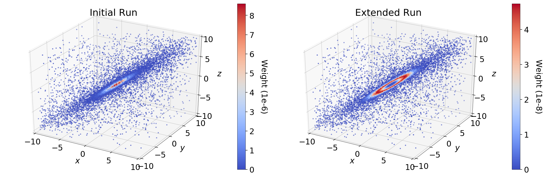
In the initial run (res1), we see that the majority of the importance weight \(\hat{p}_i\) is concentrated near the mode; in the extended run, however, it is instead concentrated in a ring around the mode. This behavior represents the fundamental compromise between the likelihood \(\mathcal{L}_i\) and the change in prior volume \(\Delta X_i\). The stark difference in the distribution of weights between the two samples is driven entirely by differences in \(\Delta X_i\). In the extended run (res2), the distribution of weights directly follows the shape expected from the “typical set” (see Typical Sets for additional discussion).

By contrast, since the final set of live points after \(N\) samples are uniformly sampled within \(X_{i=N}\), the expected change in the prior volume is constant. This leads to linear (rather than exponential) compression of the remaining prior volume, where the weight assigned to the live point with the \(k\)-th lowest likelihood is then \(\propto f(\mathcal{L}_{N+k}) \, X_N\). In the case where there is a significant portion of prior volume remaining (as with res1), this leads to extremely rapid traversal of the remaining prior volume and hence large importance weights.

dyplot

To avoid introducing an excessive burden on typical users, dynesty comes with a variety of built-in plotting utilities in the plotting module. These include a variety of generic summary plots as well as ways of visualizing bounding distributions throughout the course of a run. We can import them using:

from dynesty import plotting as dyplot

The dyplot alias will be used for convenient shorthand throughout the remainder of the documentation. While some basic usage will be demonstrated below, please see the API for additional details.

One important note is that the default credible intervals in all plotting utilities are defined to be 95% (2-sigma) rather than 68% (1-sigma). This is a deliberate choice meant to highlight more realistic uncertainties (1-in-3 vs 1-in-20 chances) and better capture possible secondary solutions at the 2.5% level rather than the roughly 16% level.

Summary Plots

One of the most direct ways of visualizing how Nested Sampling computes the evidence is by examining the relationship between the prior volume \(\ln X_i\) and:

the (effective) iteration \(i\), which illustrates how quickly/slowly our samples are compressing the prior volume,
the likelihood \(\mathcal{L}_i\), to see how smoothly we sample “up” the likelihood distribution to the maximum likelihood (ML) estimate,
the importance weight \(\hat{p}_i\), showcasing where the bulk of the posterior mass is located (i.e. the typical set), and
the evidence \(\hat{\mathcal{Z}}_i\), to see where most of the contribution to the evidence (and its respective errors) are coming from.

A summary (run) plot showcasing these features can be generated using runplot(). As an example, a summary plot for res2 comparing it to the actual analytic \(\ln \mathcal{Z}\) evidence solution can be generated using:

lnz_truth = ndim * -np.log(2 * 10.)  # analytic evidence solution
fig, axes = dyplot.runplot(res2, lnz_truth=lnz_truth)  # summary (run) plot

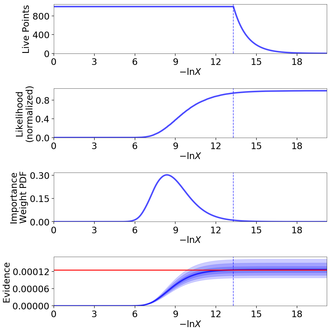
Up until we recycle our final set of live points (see Basic Algorithm), as indicated by the dashed lines, the relationship between \(\ln X_i\) and \(i\) is linear (i.e. prior volume compression is exponential). Afterwards, however, it stretches out, rapidly traversing the remaining prior volume in linear fashion. Comparing the general shape of the likelihood and importance weights subplots also highlight how the typical set is as much a function of \(\Delta X_i\) as \(\mathcal{L}_i\): although contributions initially increase as the likelihood increases, they quickly fall as the ML region encompasses increasingly smaller effective volumes.

Trace Plots

Another common way to visualize the results of many sampling algorithms is to generate a trace plot showing the evolution of particles (and their marginal posterior distributions) in 1-D projections. This can be done using the traceplot() function, which plots a combination of particle positions as a function of \(\ln X\) (colored by importance weight) and the corresponding 1-D marginalized posterior:

fig, axes = dyplot.traceplot(res2, truths=np.zeros(ndim),
                             truth_color='black', show_titles=True,
                             trace_cmap='viridis', connect=True,
                             connect_highlight=range(5))

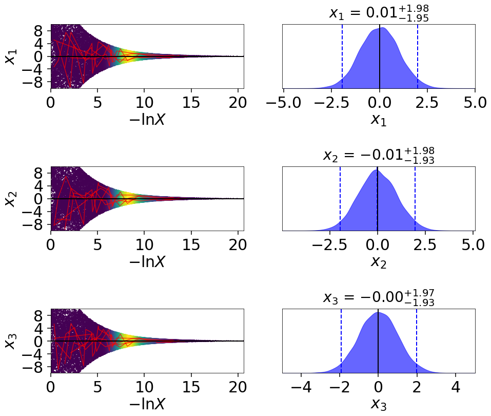
By default, traceplot() returns the samples color-coded by their relative posterior mass and the 1-D marginalized posteriors smoothed by a Normal (Gaussian) kernel with a standard deviation set to ~2% of the provided range (which defaults to the 5-sigma bounds computed from the set of weighted samples). It also can overplot input truth vectors as well as highlight specific particle paths (shown above) to inspect the behavior of individual particles. These can be useful to qualitatively identify problematic behavior such as strongly correlated samples.

Corner Plots

In addition to trace plots, another common way to visualize (weighted) samples is using corner plots (also called “triangle plots”), which show a combination of 1-D and 2-D marginalized posteriors. dynesty supports several corner plotting functions. The most straightforward is cornerpoints(), which simply plots the sample positions colored according to their estimated posterior mass if kde=True and raw importance weights if kde=False. An example highlighting the difference between the two runs is shown below:

# initialize figure
fig, axes = plt.subplots(2, 5, figsize=(25, 10))
axes = axes.reshape((2, 5))  # reshape axes

# add white space
[a.set_frame_on(False) for a in axes[:, 2]]
[a.set_xticks([]) for a in axes[:, 2]]
[a.set_yticks([]) for a in axes[:, 2]]

# plot initial run (res1; left)
fg, ax = dyplot.cornerpoints(res1, cmap='plasma', truths=np.zeros(ndim),
                             kde=False, fig=(fig, axes[:, :2]))

# plot extended run (res2; right)
fg, ax = dyplot.cornerpoints(res2, cmap='viridis', truths=np.zeros(ndim),
                             kde=False, fig=(fig, axes[:, 3:]))

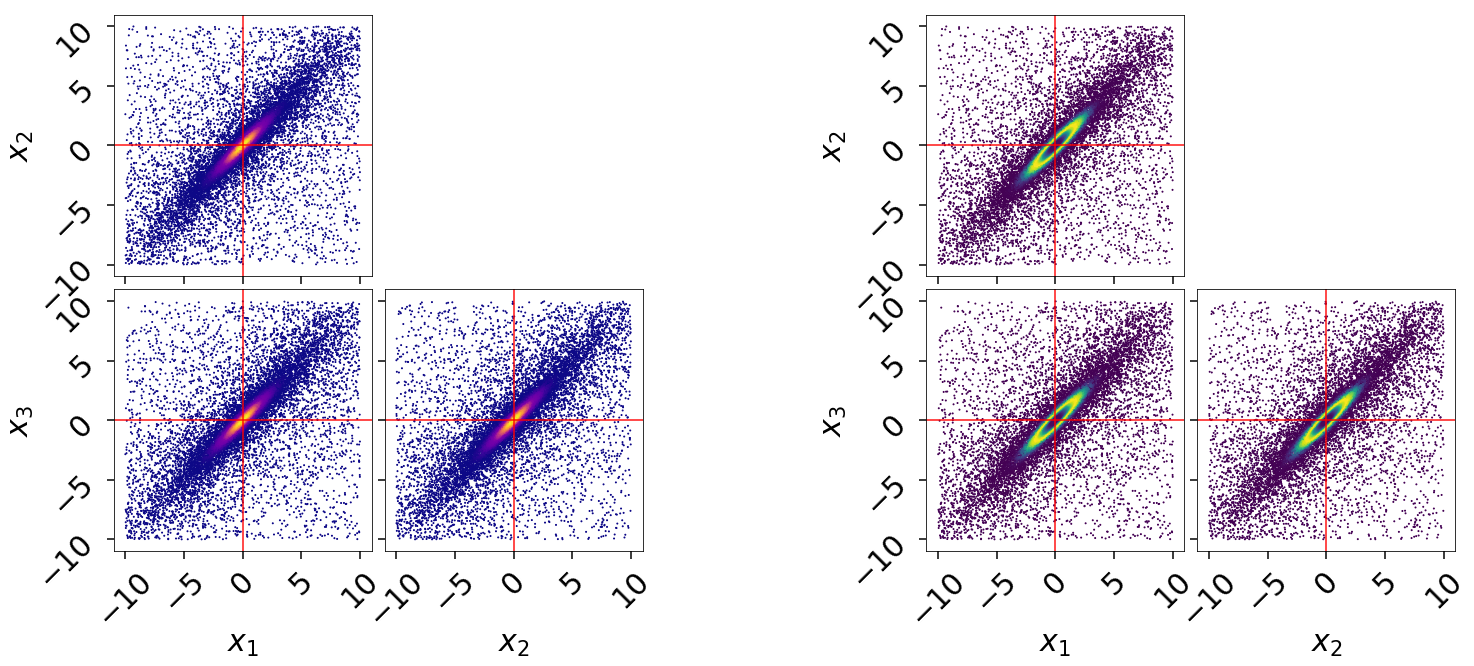
Just by looking at our projected samples, it is apparent that the results from the extended run res2 does a much better job of localizing the overall distribution compared to res1. We can get a better qualitative and quantitative handle on this by plotting the marginal 1-D and 2-D posterior density estimates using cornerplot() as:

# initialize figure
fig, axes = plt.subplots(3, 7, figsize=(35, 15))
axes = axes.reshape((3, 7))  # reshape axes

# add white space
[a.set_frame_on(False) for a in axes[:, 3]]
[a.set_xticks([]) for a in axes[:, 3]]
[a.set_yticks([]) for a in axes[:, 3]]

# plot initial run (res1; left)
fg, ax = dyplot.cornerplot(res1, color='blue', truths=np.zeros(ndim),
                           truth_color='black', show_titles=True,
                           max_n_ticks=3, quantiles=None,
                           fig=(fig, axes[:, :3]))

# plot extended run (res2; right)
fg, ax = dyplot.cornerplot(res2, color='dodgerblue', truths=np.zeros(ndim),
                           truth_color='black', show_titles=True,
                           quantiles=None, max_n_ticks=3,
                           fig=(fig, axes[:, 4:]))

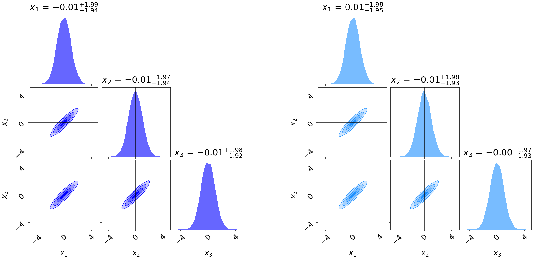
Similar to runplot(), the marginal distributions shown are by default smoothed by 2% in the specified range using a Normal (Gaussian) kernel. Notice that even though our original run res1 gave similar evidence estimates to the extended run res2, it gives somewhat “noisier” estimates of the posterior.

Bounding Distribution Plots

To visualize how we’re sampling in nested “shells”, we can look at the evolution of our bounding distributions in a given 2-D projection over the course of a run. The boundplot() function allows us to look at the bounding distributions from two different perspectives: the bounding distribution used when proposing new live points at a specific iteration (specified using it), or the bounding distribution that a given dead point originated from (specified using idx). While boundplot() natively plots in the space of the unit cube, if a specified prior_transform() is passed all samples are instead converted to the original (native) model space.

Using boundplot(), we can examine the evolution of the bounding distributions over a given run via:

# initialize figure
fig, axes = plt.subplots(2, 3, figsize=(15, 10))

# plot 6 snapshots over the course of the run
for i, a in enumerate(axes.flatten()):
    it = int((i+1)*res2.niter/8.)
    # overplot the result onto each subplot
    temp = dyplot.boundplot(res2, dims=(0, 1), it=it,
                            prior_transform=prior_transform,
                            max_n_ticks=3, show_live=True,
                            span=[(-10, 10), (-10, 10)],
                            fig=(fig, a))
    a.set_title('Iteration {0}'.format(it), fontsize=26)
fig.tight_layout()

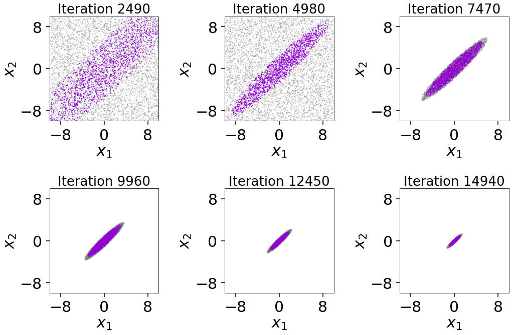
The figure illustrates that we first begin sampling directly from the unit cube. After the conditions in first_update are satisfied, we then switch over to the default multi-ellipsoidal bounding distributions. We see that these are able to adapt well to the target distribution over time, ensuring we continue to sample efficiently. We can also see the impact of bootstrapping on the bounding ellipsoids since they always remain slightly larger than the set of live points. While it slightly decreases the overall sampling efficiency, this shows how the procedure helps to ensure no likelihood is “left out” during the course of the Nested Sampling run.

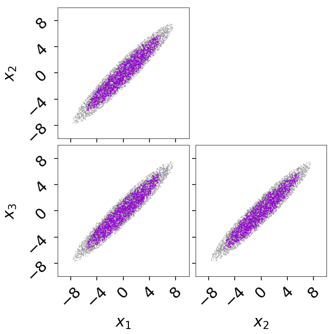
Alternately, we can generate a corner plot of the bounding distribution using cornerbound() via:

fig, axes = dyplot.cornerbound(res2, it=5000,
                              prior_transform=prior_transform,
                              show_live=True,
                              span=[(-10, 10), (-10, 10)])

Basic Post-Processing

In addition to plotting, dynesty also contains some post-processing utilities in the utils module. In many cases, a rough approximation of the posterior using the first two moments (mean and covariance) can be useful. These can be computed from the set of (weighted) samples using the mean_and_cov() function:

from dynesty import utils as dyfunc

samples, weights = res2.samples, res2.importance_weights()
mean, cov = dyfunc.mean_and_cov(samples, weights)

Runs can also be resampled to give a new set of points with equal weights, similar to MCMC methods, using the resample_equal() function:

new_samples = res2.samples_equal()

See Nested Sampling Errors for some additional discussion and demonstration of more functions.